•
Author: Yannis Nevers •
∞
I am excited to introduce our preprint for our new tool OMArk. We hope our software will help fill a gap in assessing the quality of gene annotation sets.
Many studies directly rely on the protein-coding gene repertoires (“proteomes”) predicted from genome assemblies to perform their comparisons. Doing so, they rely on the assumption that the predicted gene content of all genomes are of homogeneous quality and an accurate reflection of reality. Yet in practice, this assumption is rarely met, with protein-coding genes often missing or fragmented in the reported proteomes, non-coding sequences wrongly annotated as coding genes by gene predictors, or contamination from other species wrongly included among the reported sequences.
Why a new proteome quality tool?
Our new method, OMArk, provides a way to easily and comprehensively measure different aspects of proteome quality: completeness of the gene repertoire, consistency of the included genes at the taxonomic level, whether they have doubtful gene structures, and presence or not of inter or intra-domain contamination. Furthermore, contrary to existing methods, OMArk does not rely on a manual selection of reference dataset; instead, it automatically identifies the most likely taxonomic classification of the test proteomes. It can thus process any test proteome across the tree of life using a universal reference database.
Conceptual overview of OMArk (left) and how the innovative consistency assessment is computed (right).
OMArk is accurate and provides new insights
We performed extensive validation of the method by introducing controlled amounts of noise, fragmentation and contamination to reference proteomes and accurately estimating these amounts using OMArk. We also performed a large-scale analysis of 1805 eukaryotic UniProt Reference Proteomes with our software and were able to detect unambiguous cases of quality issues, either caused from incompleteness, contamination, or inclusion of translated non-coding sequences. In the most extreme case, we found a plant proteome with contamination from eight different species—fungi and bacteria.
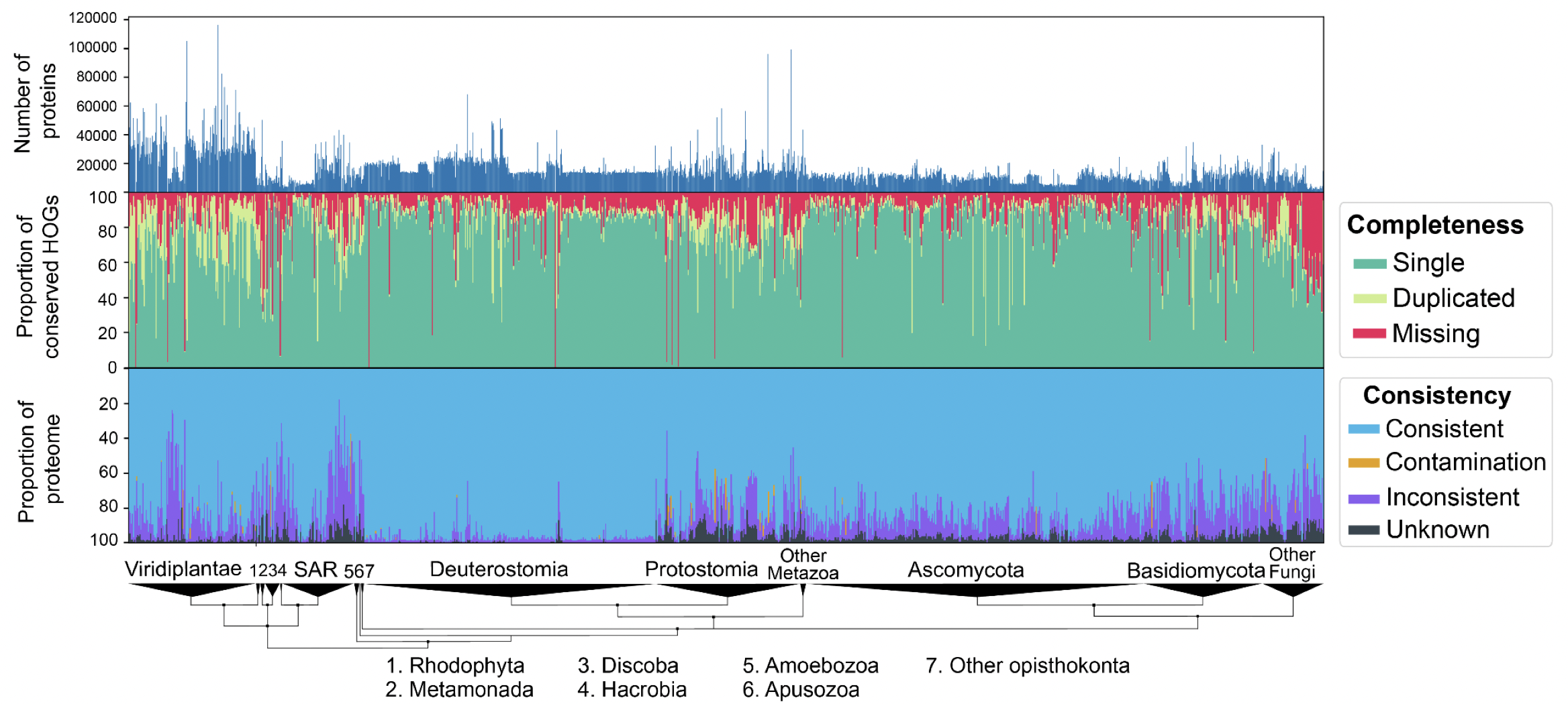
OMArk results on 1805 Eukaryotic proteomes from UniProt. Interactively check results on the OMArk webserver, e.g. for the current cowpea weevil reference proteome.
Why does the consistency metric matter? For example, comparing the Ensembl gene set for two assemblies of Bombus impatiens. We can detect a major improvement in consistency (including contamination removal) for a similar completeness.
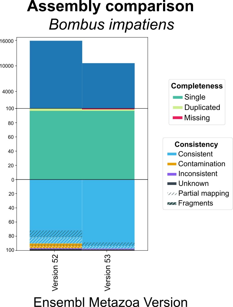
OMArk can reveal improvements in genome assemblies/annotations even if completeness has not substantially changed.
OMArk is quick and easy to run
OMArk can be easily used as a command line tool or on our OMArk webserver. On the webserver, you can submit a FASTA file of your proteome and get results in about 30 minutes. Nothing more required. You can visualize the results and directly compare it to precomputed results from closely related species (UniProt reference proteomes).
More details can be found in the preprint linked below. Please let us know how the tool works for you!
Reference
Yannis Nevers, Alex Warwick Vesztrocy, Victor Rossier, Clément-Marie Train, Adrian Altenhoff, Christophe Dessimoz, Natasha M Glover
Quality assessment of gene repertoire annotations with OMArk
Nature Biotechnology 2024 doi:10.1038/s41587-024-02147-w
•
Author: Natasha Glover •
∞
Got newly sequenced genomes with protein annotations? Need to quickly and easily define the homologous relationships between the genes?
OMA Standalone is a software developed by our lab which can be used to infer homologs from whole genomes, including orthologs, paralogs, and Hierarchical Orthologous Groups (Altenhoff et al 2019).
The OMA Standalone algorithm works like this:
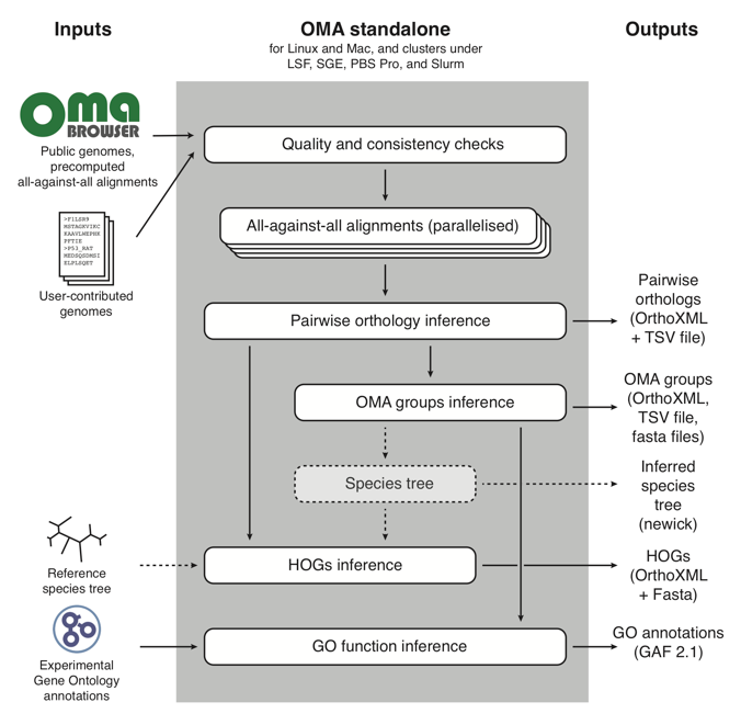
In short, it takes as input user-contributed custom genomes (with the option of combining them with reference genomes already in the OMA database), and proceeds through three main parts:
- Quality and consistency checks of the genomes that will be used to run OMA Standalone;
- All-against-all alignments of every protein sequence to all other protein sequences;
- Orthology inference, in the form of: pairwise orthologs, OMA Groups, and Hierarchical Orthologous Groups (HOGs). For more information on these types of orthologs output by OMA, see OMA: A Primer (Zahn-Zabal et al. 2020).
Although the OMA Standalone is well-documented and straightforward, one of the challenges can be running it on an High Performance Cluster (HPC).
In order to understand the bare necessities needed to run OMA Standalone, we wrote an OMA Standalone Cheat Sheet, which you can download and follow the step-by-step instructions on running the software on an HPC. We use the cluster Wally as an example, as that is one of the HPCs here at the University of Lausanne. Wally uses SLURM as the scheduler for submitting jobs, so all the examples will be shown with that. We plan in the future to provide additional information on running with other schedulers, such as LSF or SGE. In the Cheat Sheet, you will find tips, hints, commands, and example scripts to run OMA Standalone on Wally.
Additionally, we prepared a video which walks the user through the process of running OMA Standalone from start to finish, including:
- Downloading the software
- Preparing your genomes for running
- Editing the necessary parameters file
- Creating the job scripts and
- Submitting your jobs
The video can be found on our lab’s YouTube channel, at OMA standalone: how to efficiently identify orthologs using a cluster, and is also embedded here for your convenience:
We hope these resources can be helpful if you need help getting started running OMA Standalone. But don’t forget, there is also plenty of information that can be found on the OMA Standalone webpage or in the OMA Standalone paper. If all else fails, don’t hesitate to contact us on Biostars.
References
- Altenhoff, A. M. et al. OMA standalone: orthology inference among public and custom genomes and transcriptomes. Genome Res. 29, 1152–1163 (2019).
- Zahn-Zabal, M., Dessimoz, C. & Glover, N. M. Identifying orthologs with OMA: A primer. F1000Res. 9, 27 (2020).
•
Author: Christophe Dessimoz •
∞
We just submitted a paper to Nucleic Acids Research Web Server issue. As it
turns out, the editor requires a bibliography with links to DOI, PubMed, and PubMedCentral entries.
This is a brief tutorial to generate such a bibliography from a bibtex file
which contains the relevant entries, loosely based on the explanations
provided in this TeX StackExchange entry.
Generating the bibtex file
In the lab, we mainly use Paperpile as bibliography management system, but most system allow to export records in bibtex format. If available, Paperpile includes DOI, PubMed IDs, and PubMedCentral IDs as follows:
@ARTICLE{Glover2019-xs,
    title    = "{Assigning confidence scores to homoeologs using fuzzy logic}",
    author   = "Glover, Natasha M and Altenhoff, Adrian and Dessimoz, Christophe",
    journal  = "PeerJ",
    volume   =  6,
    pages    = "e6231",
    year     =  2019,
    doi      = "10.7717/peerj.6231",
    pmid     = "30648004",
    pmc      = "PMC6330999"
}
In this example, we store the bibliography in a file named ref.bib.
Extending biblatex to include PMID and PMC links in the bibliography
DOI are already supported by most bibliography systems. To also include PMID and PMCIDs, the trick is to use the flexible BibLatex package.
In a separate definition file, which we named adn.dbx, add the
additional definitions for PMID and PMCIDs.
\DeclareDatamodelFields[type=field,datatype=literal]{
    pmid,
    pmc,
}
We can now include this file in the library definition in the main LaTeX file
(in the preamble, i.e. before \begin{document}, and define the
links to PubMed and PubMedCentral entries:
\usepackage[backend=biber,style=authoryear,datamodel=adn]{biblatex}
\DeclareFieldFormat{pmc}{%
  PubMedCentral\addcolon\space
  \ifhyperref
    {\href{http://www.ncbi.nlm.nih.gov/pmc/articles/#1}{\nolinkurl{#1}}}
    {\nolinkurl{#1}}}
\DeclareFieldFormat{pmid}{%
  PubMed ID:\addcolon\space
  \ifhyperref
    {\href{https://www.ncbi.nlm.nih.gov/pubmed/#1}{\nolinkurl{#1}}}
    {\nolinkurl{#1}}}
\renewbibmacro*{finentry}{%
  \printfield{pmid}%
  \newunit
  \printfield{pmc}%
  \newunit
  \finentry}
\addbibresource{ref.bib}
We can generate the bibliography by citing every paper using the \cite{} command, and printing the bibliography.
\cite{Glover2019-xs}
\newpage
\printbibliography
Polishing: highlighting the links with colour
To make the links more visible, define the hyperref package
accordingly:
\usepackage[colorlinks]{hyperref}
OK, thanks but could I just have the files please?
Of course! Here they are.
•
Author: Natasha Glover •
∞
You’ve wrapped up the research on project. You’ve gotten good results. It’s time to publish them—your PhD/postdoc/career depends on it.
But you’re drawing a blank. Staring at the screen for hours, not knowing how to get started, and the only thing you can produce is an empty document. One of the most daunting tasks for young scientists is writing and publishing a paper, especially the first one.
In the context of a tutorial of the UNIL Quantitative Biology PhD Program, I prepared a series of three short videos featuring interviews with professors on tips to successfully publish a scientific paper. These videos were aimed towards PhD students, but contain useful advice for anyone, at any stage of their career. Here’s what they had to say:
Part 1: the writing process
Part 2: the journal selection
Part 3: responding to reviewers
•
Author: Natasha Glover •
∞
All living organisms descended from a common ancestor, and therefore all living organisms have some genes in common. Therefore, we can take any two species on the tree of life and find out what set of genes were present in the common ancestor of the two species by looking for the genes that they still share to this day. When two species are closely related, i.e. close together on the tree of life, we can observe that much of their genome is the same. But what do I mean by “same”, and what do I mean by “shared”?
Genomes are complex, with many layers of control (DNA-level, RNA-level, protein-level, epigenetic level, alternative splicing-level, protein-protein interaction level, transposable element-level, etc). Because of this complexity, there could be many ways to compare the genomes of two different species to determine which portion of the genome is shared.
In this blog post, when I refer to “shared” parts of the genome, I’m referring to orthologs, which are genes in different species that started diverging due to a speciation event. Orthologs can be inferred from complete genome sequences, and there are many different methods to do this. In particular, I will focus on the Dessimoz lab’s method and database, Orthologous MAtrix, or OMA. OMA uses protein sequences from whole genome annotations to compute orthologs between over 2000 species. The OMA algorithm is graph-based, compares all protein sequences to all others to find the closest between two genomes, allows for duplicates, and uses information from related genomes to improve the calling. OMA is available at https://omabrowser.org/.
It’s quite well-publicized that humans and chimps are extremely similar in terms of gene content, which is why they could be considered our evolutionary cousins1. However, when two species are more distantly related, there is less of their genomes which are the same. But how distant can we go in the tree of life and still see the same genes between different species? For example, how many genes do I (a human) have in common with a plant? Can we even detect orthologs between two species so evolutionarily distant? And if so, what biological/functional role do these genes play?
In this blog post, I will show how to use OMA and some of its tools to find out how much of the human genome we share with plants. There are many different plant species with their genomes’ sequenced, so I will use the extensively-studied model species Arabidopsis thaliana as the representative plant to compare the human protein-coding genes to.
Setup
For the remainder of this blog post, I will show how to use the OMA database, accessed via the python REST API, to get ortholog pairs between two genomes.
In python, I use the requests library to send queries for information to the server housing the OMA database. Pandas is a well-known python library for working with dataframes, so I will use that for analysis. For more information, see:
Let’s start our python code by importing libraries:
import requests
import json
import pandas as pd
The OMA API is accessible from the following link, so we will save it for later use in our code:
api_url = "https://omabrowser.org/api"
Getting pairwise orthologs with the OMA API
Pairwise orthologs are computed between all pairs of species in OMA as part of the normal OMA pipeline. Accessing the data will result in a list of pairs of genes, one from one species and the other from the other species. Any one gene may be involved in several different pairs, depending of if its ortholog has undergone duplication or not.
It is important to note that here we are only using pairs of orthologs. In OMA, we report several types of orthologs, namely pairs of orthologs or groups of orthologs (Hierarchical Orthologous Groups (HOGs). We use the pairs as the basis for building HOGs, which aggregates orthologous pairs together into clusters at different taxonomic levels. Some ortholog pairs are removed, and some new pairs are inferred when creating HOGs. Therefore, the set of orthologs deduced from HOGs will be slightly different than the set of orthologs purely from the pairs.
Here we will use the API to request all the pairwise orthologs between Homo sapiens and Arabidopsis thaliana. OMA uses either the NCBI taxon identifier or the 5-letter UniProt species code to identify species. I will use the UniProt codes, which are “HUMAN” and “ARATH.” To request the ortholog pairs between HUMAN and ARATH, the request would simply look like:
requests.get(api_url + '/pairs/HUMAN/ARATH/')
However, when sending a request that returns long lists, i.e. lists of thousands of genes, the OMA API uses pagination. This means all the results won’t be returned at once, but sequentially page by page, with only 100 results per page. This is a safeguard to make sure the OMA servers don’t get overloaded with requests. Here I show a simple workaround to get all of the pairs.
Get all pairs
genome1 = "HUMAN"
genome2 = "ARATH"

#get first page
response = requests.get(api_url + '/pairs/{}/{}/'.format(genome1, genome2))

#use the header to calculate total number of pages
total_nb_pages = round(int(response.headers['X-Total-Count'])/100)
print("There are {} pages that need to be requested.".format(total_nb_pages))

> There are 128 pages that need to be requested.
Since we want all the pages, not just the first one, we have to use a loop to go through and request all the pages.
#get responses for all pages
responses = []
for page in range(1, total_nb_pages + 1):
    tmp_response = requests.get(api_url + '/pairs/{}/{}/'.format(genome1, genome2)+"?page="+str(page))
    responses.append(tmp_response.json())

#some basic tidying up so we only have a list of pairs at the end
pairs = []
for response in responses:
    for pair in response:
        pairs.append(pair)

#Example of a pair
pairs[0]

> {'entry_1': {'entry_nr': 8066469,
>   'entry_url': 'https://omabrowser.org/api/protein/8066469/',
>   'omaid': 'HUMAN00009',
>   'canonicalid': 'NOC2L_HUMAN',
>   'sequence_md5': 'dc91b2521daf594037a6c318f3b04d5a',
>   'oma_group': 840151,
>   'oma_hog_id': 'HOG:0420566.4b.15b.5a.3b',
>   'chromosome': '1',
>   'locus': {'start': 944694, 'end': 959240, 'strand': -1},
>   'is_main_isoform': True},
>  'entry_2': {'entry_nr': 12384097,
>   'entry_url': 'https://omabrowser.org/api/protein/12384097/',
>   'omaid': 'ARATH12334',
>   'canonicalid': 'NOC2L_ARATH',
>   'sequence_md5': 'f19ac310a5e56443f2ce0e4e832addb3',
>   'oma_group': 840151,
>   'oma_hog_id': 'HOG:0420566.1c',
>   'chromosome': '2',
>   'locus': {'start': 7928254, 'end': 7931851, 'strand': 1},
>   'is_main_isoform': True},
>  'rel_type': '1:1',
>  'distance': 138.0,
>  'score': 1094.969970703125}
We can see that the data is in the form of a big list of pairs, with each pair being a dictionary. In this dictionary, one key is entry_1, which is the human gene, and the second key is entry_2, which is the arabidopsis gene. The values for each of these keys are dictionaries with information about the gene. Additionally, there are other key value pairs in the pair dictionary which gives information computed about the pair, such as rel_type, distance, and score (will be explained later).
Make dataframe with all pairs
I personally like to work with pandas because I find it easy to use, so I will import the information about the pairs into a dataframe.
#use pandas to make dataframe
df = pd.DataFrame.from_dict(pairs)

def make_columns_from_entry_dict(df, columns_to_make):
    '''Parses out the keys from the entry dictionary and adds them to the dataframe
    with an appropriate column header.'''

    genome1 = df['entry_1'][0]['omaid'][:5]
    genome2 = df['entry_2'][0]['omaid'][:5]

    df[genome1+"_"+columns_to_make] = df.apply(lambda x: x['entry_1'][columns_to_make], axis=1)
    df[genome2+"_"+columns_to_make] = df.apply(lambda x: x['entry_2'][columns_to_make], axis=1)

    return df

#clean up the columns of the entry_1 and entry_2 dictionaries
df = make_columns_from_entry_dict(df, "omaid")
df = df[['HUMAN_omaid','ARATH_omaid','rel_type','distance','score']]

#Here's a snippet of the dataframe
df[:10]
|
HUMAN_omaid |
ARATH_omaid |
rel_type |
distance |
score |
| 0 |
HUMAN00009 |
ARATH12334 |
1:1 |
138.0 |
1094.969971 |
| 1 |
HUMAN00029 |
ARATH38493 |
1:1 |
168.0 |
246.330002 |
| 2 |
HUMAN00032 |
ARATH38034 |
1:1 |
69.0 |
773.869995 |
| 3 |
HUMAN00034 |
ARATH39850 |
m:n |
140.0 |
635.900024 |
| 4 |
HUMAN00034 |
ARATH33319 |
m:n |
144.0 |
655.409973 |
| 5 |
HUMAN00034 |
ARATH01678 |
m:n |
137.0 |
723.580017 |
| 6 |
HUMAN00034 |
ARATH07547 |
m:n |
134.0 |
761.450012 |
| 7 |
HUMAN00036 |
ARATH01479 |
1:1 |
103.0 |
554.590027 |
| 8 |
HUMAN00037 |
ARATH10852 |
1:1 |
60.0 |
2325.889893 |
| 9 |
HUMAN00052 |
ARATH02626 |
1:1 |
95.0 |
328.959991 |
Here you can see that each row is a pair of orthologs, with some information about each. The rel_type is the relationship cardinality, between the orthologs. 1:1 means only one ortholog in human found in arabidopsis, whereas 1:m would mean it duplicated in ARATH. m:n means there were lineage-specific duplications on both sides.
How many pairs between HUMAN and ARATH?
print("There are {} pairs of orthologs between {} and {}.".format(len(df), genome1, genome2))

> There are 12792 pairs of orthologs between HUMAN and ARATH.
What percentage is this of the human genome? What percentage of the Arabidopsis genome? To answer this we need to 1) Get the number of genes in each genome that this represents, because there can be more than 1 pair of orthologs per gene. 2) We also need to get the total number of genes per genome.
First we get the number of genes for each species that has at least one ortholog, using the dataframe from above. We don’t have to worry about alternative splic variants (ASVs) because OMA chooses a representative isoform when computing orthologs.
human_proteins_with_ortholog = set(df['HUMAN_omaid'].tolist())
print("There are {} genes in {} with at least 1 ortholog in {}.".\
      format(len(human_proteins_with_ortholog), "HUMAN","ARATH"))

arath_proteins_with_ortholog = set(df['ARATH_omaid'].tolist())
print("There are {} genes in {} with at least 1 ortholog in {}.".\
      format(len(arath_proteins_with_ortholog), "ARATH","HUMAN"))

> There are 3769 genes in HUMAN with at least 1 ortholog in ARATH.
> There are 5177 genes in ARATH with at least 1 ortholog in HUMAN.
Get the genomes of HUMAN and ARATH
Now we will again use the API to get all the proteins in the genome. (See https://omabrowser.org/api/docs#genome-proteins). Here I will write a function using the same procedure as above to deal with pagination.
#Use the API to get all the human genes
def get_all_proteins(genome):
    '''Gets all proteins using OMA REST API'''
    responses = []
    response = requests.get(api_url + '/genome/{}/proteins/'.format(genome))
    total_nb_pages = round(int(response.headers['X-Total-Count'])/100)
    for page in range(1, total_nb_pages + 1):
        tmp_response = requests.get(api_url + '/genome/{}/proteins/'.format(genome)+"?page="+str(page))
        responses.append(tmp_response.json())

    proteins = []
    for response in responses:
        for entry in response:
            proteins.append(entry)
    return proteins


human_proteins = get_all_proteins("HUMAN")

#Here is an example entry
human_proteins[0]

> {'entry_nr': 8066461,
>  'entry_url': 'https://omabrowser.org/api/protein/8066461/',
>  'omaid': 'HUMAN00001',
>  'canonicalid': 'OR4F5_HUMAN',
>  'sequence_md5': 'df953df7a11ee7be5484e511551ce8a4',
>  'oma_group': 650473,
>  'oma_hog_id': 'HOG:0361626.2a.7a',
>  'chromosome': '1',
>  'locus': {'start': 69091, 'end': 70008, 'strand': 1},
>  'is_main_isoform': True}
It is important to note that this list of genes/proteins includes ASVs for many species. Therefore we need to take care to remove them to have one represenative isoform per gene. We can do this by filtering the list of entries based on the ‘is_main_isoform’ key. Here is a small function to do that.
#get canonical isoform
def get_canonical_proteins(list_of_proteins):
    proteins_no_ASVs = []
    for protein in list_of_proteins:
        if protein['is_main_isoform'] == True:
            proteins_no_ASVs.append(protein)
    return proteins_no_ASVs

print("HUMAN\n-----")
print("The number of genes before removing alternative splice variants: {}".format(len(human_proteins)))

human_proteins_no_ASVs = get_canonical_proteins(human_proteins)

print("The number of genes after removing alternative splice variants: {}".format(len(human_proteins_no_ASVs)))


> HUMAN
> -----
> The number of genes before removing alternative splice variants: 30700
> The number of genes after removing alternative splice variants: 20152


#Do the same for ARATH
print("ARATH\n-----")
arath_proteins = get_all_proteins("ARATH")

print("The number of genes before removing alternative splice variants: {}".format(len(arath_proteins)))
arath_proteins_no_ASVs = get_canonical_proteins(arath_proteins)
print("The number of genes after removing alternative splice variants: {}".format(len(arath_proteins_no_ASVs)))

> ARATH
> -----
> The number of genes before removing alternative splice variants: 40999
> The number of genes after removing alternative splice variants: 27627
Proportion of the genomes which have orthologs in the other
Now that we have all the necessary information we can see what percentage of the human and arabidopsis genomes are shared, in terms of proportion of genes with at least 1 ortholog in the other species.
print("The percentage of genes in {} with at least 1 ortholog in {}: {}%"\
      .format("HUMAN", "ARATH", \
              round((len(human_proteins_with_ortholog)/len(human_proteins_no_ASVs)*100), 2)))

print("The percentage of genes in {} with at least 1 ortholog in {}: {}%"\
      .format("ARATH", "HUMAN", \
              round((len(arath_proteins_with_ortholog)/len(arath_proteins_no_ASVs)*100), 2)))

> The percentage of genes in HUMAN with at least 1 ortholog in ARATH: 18.7%
> The percentage of genes in ARATH with at least 1 ortholog in HUMAN: 18.74%
So the answer to the original questions is that BOTH humans and arabidopsis have 18.7% of their genome shared with each other. A weird coincidence that it turns out to be the same proportion of both genomes!
Conclusion
Using the OMA database for orthology inference, we found that:
- There are 12792 pairs of orthologs between HUMAN and ARATH.
- There are 3769 genes in human that have at least 1 ortholog in arabidopsis.
- There are 5177 genes in arabidopsis that have at least 1 ortholog in human.
- These numbers represent about 19% of both genomes.
Therefore, we can conclude that over the course of evolution since the animal and plant lineages split (~1.5 billion years ago2), about 19% of the protein-coding genes remain and are able to be detected by OMA.
Stay tuned for the next blog post, where I will show what are the functions of these shared genes!
References
- Chimpanzee Sequencing and Analysis Consortium. Initial sequence of the chimpanzee genome and comparison with the human genome. Nature 437, 69–87 (2005). DOI: https://doi.org/10.1038/nature04072
- Wang, D. Y., Kumar, S. & Hedges, S. B. Divergence time estimates for the early history of animal phyla and the origin of plants, animals and fungi. Proc. Biol. Sci. 266, 163–171 (1999). DOI: 10.1098/rspb.1999.0617
•
Author: Clement Train •
∞
(This entry was updated 19 Sep 2018 to reflect recent feature updates)
pyHam (‘python HOG analysis method’) makes it possible to extract useful information from HOGs encoded in standard OrthoXML format. It is available both as a python library and as a set of command-line scripts. Input HOGs in OrthoXML format are available from multiple bioinformatics resources, including OMA, Ensembl and HieranoidDB.
This post is a brief primer to pyham, with an emphasis on what it can do for you.
How to get pyHam?
pyHam is available as python package on the pypi server and
is compatible python 2 and python 3. You can easily install via
pip using the following bash command:
pip install pyham
You can check the official pyham website for
further information about how to use pyham, documentation and the source code.
What are Hierarchical Orthologous Groups (HOGs)?
You don’t know what HOGs are and you are eager to change this, we have an explanatory video about them just for you:
You can learn more about this in our previous blog post.
Where to find HOGs?
HOGs inferred on public genomes can be downloaded from the OMA orthology database. Other databases, such as Eggnog, OrthoDb or HieranoiDB also infer HOGs, but not all of these databases offer them in OrthoXML format. You can check which database serves hogs as orthoxml here. If you want to use your custom genomes to infer HOGs you can use the OMA standalone software.
In order to facilitate the use of pyHam on single gene family, we provide the option to let pyham fetch required data directly from a comptabilble databases (for now only OMA is available for this feature). The user simply have to give the id of a gene inside the gene family (HOGs) of insterest along with the name of the compatibible database where to get the data and pyHam will do the rest.
For example, if you are interest by the P_53 gene in rat (P53 rat gene page in OMA) you simply have to run the following python code to set-up your pyHam session:
my_gene_query = 'P53_RAT'
database_to_query = 'oma'
pyham_analysis = pyham.Ham(query_database=my_gene_query, use_data_from=database_to_query)
How does pyham help you investigate on HOGs?
The main features of pyHam are: (i) given a clade of interest, extract all the relevant HOGs, each of which ideally corresponds to a distinct ancestral gene in the last common ancestor of the clade; (ii) given a branch on the species tree, report the HOGs that duplicated on the branch, got lost on the branch, first appeared on that branch, or were simply retained; (iii) repeat the previous point along the entire species tree, and plot an overview of the gene evolution dynamics along the tree; and (iv) given a set of nested HOGs for a specific gene family of interest, generate a local iHam web page to visualize its evolutionary history.
What is the number of genes in a particular ancestral genome? (i)
In pyHam, ancestral genomes are attached to one specific internal node in the inputted species tree and denoted by the name of this taxon. Ancestral genes are then infered by fetching all the HOGs at the same level.
# Get the ancestral genome by name
rodents_genome = ham_analysis.get_ancestral_genome_by_name("Rodents")

# Get the related ancestral genes (HOGs)
rodents_ancestral_genes = rodents_genome.genes

# Get the number of ancestral genes at level of Rodents
print(len(rodents_ancestral_genes)
How can I figure out the evolutionary history of genes in a given genome? (ii)
pyHam provides a feature to trace for HOGs/genes along a branch that span across one or multiple taxonomic ranges and report the HOGs that duplicated on this branch, got lost on this branch, first appeared on that branch, or were simply retained. The ‘vertical map’ (see further information on map here) allows for retrieval of all genes and their evolutionary history between the two taxonomic levels (i.e. which genes have been duplicated, which genes have been lost, etc).
# Get the genome of interest
human = ham_analysis.get_extant_genome_by_name("HUMAN")
vertebrates = ham_analysis.get_ancestral_genome_by_name("Vertebrata")

# Instanciate the gene mapping !
vertical_human_vertebrates = ham_analysis.compare_genomes_vertically(human, vertebrates) # The order doesn't matter!

# The identical genes (that stay single copies)
# one HOG at vertebrates -> one descendant gene in human
vertical_human_vertebrates.get_retained())

# The duplicated genes (that have duplicated)
# one HOG at vertebrates -> list of its descendants gene in human
vertical_human_vertebrates.get_duplicated())

# The gained genes (that emerged in between)
# list of gene that appeared after vertebrates taxon
vertical_human_vertebrates.get_gained()

# The lost genes (that been lost in between)
HOG at vertebrates that have been lost before human taxon
vertical_human_vertebrates.get_lost()
How can I get an overview of the gene evolution dynamics along the tree that occured in my genomic setup? (iii)
pyHam includes treeProfile (extension of the Phylo.io tool), a tool to visualise an annotated species tree with evolutionary events (genes duplications, losses, gains) mapped to their related taxonomic range. The aim is to provide a minimalist and intuitive way to visualise the number of evolutionary events that occurred on each branch or the numbers of ancestral genes along the species tree.
# create a local treeprofile web page
treeprofile = ham_analysis.create_tree_profile(outfile="treeprofile_example.html")
As you can see in the figure above, the treeprofile is composed of the reference species used
to perform the pyham analysis. Each internal node is displayed with its related histogram of
phylogenetic events (number of genes duplicated, lost, gained, or retained) that occurred on each branch. The tree profile either display the number of genes resulting from phylogenetics events or the number of phylogenetic events on themself; the switch can be made by opening the settings panel (histogram icon on top right) and selecting between ‘genes’ or ‘events’.
How can I visualise the evolutionary history of a gene family (HOG)? (iv)
pyHam embeds iHam, an interactive tool to visualise gene family evolutionary history. It provides a way to trace the evolution of genes in terms of duplications and losses, from ancient ancestors to modern day species.
# Select an HOG
hog_of_interest = pyham_analysis.get_hog_by_id(2)

# create and export the hog vis as .html
output_filename = "hogvis_example.html"
pyham_analysis.create_hog_visualisation(hog=hog_of_interest,outfile=output_filename)
Then, you simply have to double click on the .html file to open it in your default internet browser. We provide you an example below of what you should see. A brief video tutorial on iHam is available at this URL.
iHam is composed of two panels: a species tree that allows you to select the
taonomic range of interest, a genes panel where each grey square represents an extant gene and each row a
species.
We can see for example that at the level of mammals (click on the related node and select ‘Freeze at this node’) all genes of this gene family are descendant from a single comon ancestral gene.
Now, if we look at the level of Euarchontoglires (redo the same procedure as for mammals to freeze the vis at this level) we
observe that the genes are now split by a vertical line. This vertical line separates 2 group of genes that are each descendants from a same single ancestral gene. This is the result of a duplication in between Mammals and Euarchontoglires.
This small example demonstrate the simplicity of iHam usefulness to identify evolutionary events that occured in gene families (e.g. when a duplication occured, which species have lost genes or how big genes families evolved).
•
Author: Christophe Dessimoz •
∞
You have a reference to a research paper of interest.
Perhaps this one:
Iantorno S et al, Who watches the watchmen? an appraisal of benchmarks for multiple sequence alignment, Multiple Sequence Alignment Methods (D Russell, Editor), Methods in Molecular Biology, 2014, Springer Humana, Vol. 1079. doi:10.1007/978-1-62703-646-7_4
How can you retrieve the full article?
Gold open access
If the paper is published as “gold” open access, you can download the PDF from the publisher’s website. In such cases, it’s easiest to paste the title and author names in Google and look for the first hit in the journal.
Alternatively, if you know the Digital Object Identifer (DOI) of the article, prepending http://doi.org should directly lead you to the article. In this case, the
DOI is included at the end of the citation. (If you don’t know its DOI, you can find it on the publisher’s website or in a database such as PubMed). We get:
http://doi.org/10.1007/978-1-62703-646-7_4
Unfortunately, we see that this particular paper is behind a paywall at the publisher.
Green open access
There is, however, still a chance that it might be deposited in a preprint server or in an institutional repository. This is referred to as “green” open access. One way to find out is to look at the article record in Google Scholar and look for a link in the right margin:
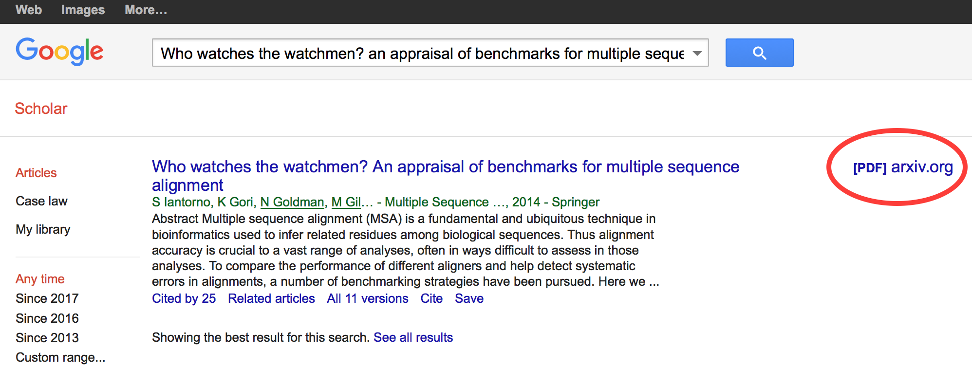
In this case, the paper is thus available on arXiv.org.
If you know the DOI, an even quicker way of looking for a deposited version is
by using the http://oadoi.org redirection tool, which works analogously to
doi.org but redirect to a green open access version whenever possible:
http://oadoi.org/10.1007/978-1-62703-646-7_4
Here, a free version of the article deposited in the UCL institutional repository is found.
If you use Chrome or Firefox, you can also use the Unpaywall browser extension to automatically get a link to green open access alternatives as you land on paywalled articles.
On the author’s homepage
Sometimes, the paper is available on the homepage of one of the authors. In
this case, a link to the preprint is provided on the homepage of the corresponding
author (item #36).
ResearchGate
Instead of an institutional homepage, some authors self-archive their articles on ResearchGate. In the case of our paper, the full-text version is indeed directly available.
And otherwise, if one of the authors is active on ResearchGate, it’s also possible to send a full-text request at the click of a button.
Pirated version off Sci-Hub
Sci-Hub serves bootleg copies of pay-walled articles. This is illegal, so I only mention it for educational purposes. This works most reliably using, again, DOIs:
http://sci-hub.tw/10.1007/978-1-62703-646-7_4
If you, purely hypothetically of course, pasted that URL in your browser, you would or would not get a PDF of the entire book in which the referenced article appears.
#icanhazpdf
It’s also possible to request full-text articles via Twitter. As described in Wikipedia, this works by tweeting the article title, its DOI, an email address (to indicate to whom the article should be sent), and the hashtag #icanhazpdf. Someone with access to the article might send a copy via email. Once the article is received, the tweet is deleted. Again, I mention this for educational purpose only—don’t break the law.

Image credit: Field of Science
Altmetrics.com wrote an interesting post on #icanhazpdf a few years ago.
Email the corresponding author
Finally, you can always ask the corresponding author by email for a copy of their article. They will happily oblige.
[Update (19 Mar 2017): added mention of unpaywall to seemlessly retrieve green open access]
•
Author: Christophe Dessimoz •
∞
One central concept in the OMA project and other
work we do to infer relationships between genes is that of Hierarchical
Orthologous Groups, or “HOGs” for the initiated.
We’ve written several papers on aspects pertaining to HOGs—how to infer
them,
how to evaluate them, them being
increasingly adopted by orthology
resources, etc.—but there is
still a great deal of confusion as to what HOGs are and why they matter.
Natasha Glover, talented postdoc in the lab, has produced a brief video to
introduce HOGs and convey why we are mad about them!
References
Altenhoff, A., Gil, M., Gonnet, G., & Dessimoz, C. (2013). Inferring Hierarchical Orthologous Groups from Orthologous Gene Pairs PLoS ONE, 8 (1) DOI: 10.1371/journal.pone.0053786
Boeckmann, B., Robinson-Rechavi, M., Xenarios, I., & Dessimoz, C. (2011). Conceptual framework and pilot study to benchmark phylogenomic databases based on reference gene trees Briefings in Bioinformatics, 12 (5), 423-435 DOI: 10.1093/bib/bbr034
Sonnhammer, E., Gabaldon, T., Sousa da Silva, A., Martin, M., Robinson-Rechavi, M., Boeckmann, B., Thomas, P., Dessimoz, C., & , . (2014). Big data and other challenges in the quest for orthologs Bioinformatics, 30 (21), 2993-2998 DOI: 10.1093/bioinformatics/btu492
 The Dessimoz Lab
blog is licensed under a Creative
Commons
Attribution 4.0 International License.
The Dessimoz Lab
blog is licensed under a Creative
Commons
Attribution 4.0 International License.