•
Author: Sina Majidian •
∞
Genomic data is expanding at a rapid pace, driven by ambitious efforts to sequence the DNA of millions of species worldwide. Comparative genomics, essentially the science of comparing genomes across species, helps us understand the evolutionary relationships between species. A key part of this is to find homologous regions, which are regions of DNA that are shared across species due to having a common ancestor.
When it comes to homologous genes, there are two main types to know about: orthologs and paralogs. Orthologs are genes that started diverging because of speciation (evolutionary branching into new species), while paralogs diverged because of gene duplication. Orthologs often have similar functions across species, which makes them extremely useful for transferring knowledge from well-studied organisms to newly sequenced ones (Nicheperovich 2022).
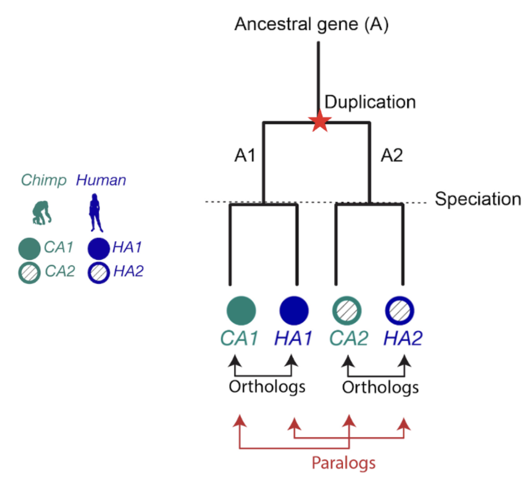
Figure 1. The relationship between two genes that share a common ancestor is called homologous, from the Greek word homologos— homos (meaning “same”) + logos (meaning “relation”). Orthologs are gene pairs that diverged due to evolutionary speciation, while paralogs are gene pairs that diverged due to a duplication event. This distinction is important because orthologs tend to have similar functions, but paralogs do not.
A bit of History!
The idea of distinguishing orthologs from paralogs goes back to Walter Fitch’s seminal work at the University of Wisconsin in 1970 (Fitch 1970). Since then, several research groups have been working on algorithms to accurately estimate orthology. One of the first contributions was the Clusters of Orthologous Groups of proteins (COGs) database, launched by NCBI in 2000, covering 21 genomes of bacteria, archaea, and eukaryotes (Tatusov 2000). More recently, the Orthofinder tool made it possible to find orthologs for a set of genomes of interest with high accuracy. This well-known software uses fast all-against-all gene comparisons with DIAMOND to group genes into orthogroups and refine them with gene trees. Earlier this year, Sonicparanoid presented its second version, which benefits from machine learning to efficiently avoid unnecessary all-against-all alignments, which makes it even faster. All these exciting advancements highlight the thriving community that works in the field of orthology and comparative genomics.
The OMA (Orthologous MAtrix) project came along in 2004 as a method and database for identifying orthologs across genomes (Dessimoz et al. 2005). The original OMA algorithm uses all-against-all gene comparisons with Smith-Waterman to find homologous sequences and then infers orthology relationships from there. Since 2010, Adrian Altenhoff has been the OMA project manager and OMA is hosted at the Comparative Genomics lab, led by Christophe Dessimoz and Natasha Glover. In 2017, Clément Train, a talented PhD student in the lab, took things to the next level with OMA algorithm 2.0, which delivered high precision in orthology inference (Train et al. 2017). Fast forward to today, the OMA Browser has seen 24 major updates where all the orthology data of around 3000 genomes is now presented for easy access with visualization innovations for phylostratigraphy, synteny and gene information (Altenhoff et al. 2024). Along the way, OMA also became a core resource supported by the SIB Swiss Institute of Bioinformatics.
In 2021, I joined the Comparative Genomics lab in Lausanne as a postdoc, took a leap of faith and started working on developing a new algorithm for orthology. The goal was to make it work for several thousands of species, basically scaling to the tree of life—something that’s really needed these days. At first, it felt quite overwhelming as there were several efficient ortholog inference tools such as Panther, OrthoMCL, Orthofinder, Sonicparanoid, Ensembl compara, Domainoid, MetaPhOrs, TOGA and GETHOGS (to name only a few) that are being maintained rigorously and regularly. The developer of these tools made great contributions to the field, and the huge number of comparative genomics studies over the years wouldn’t have been possible without these softwares. Their intricate design and comprehensive algorithms are accurate and efficient, making it hard to imagine advancing the field even further.
On top of that, I was new to the field—my PhD was on diploid and polyploid haplotype phasing using DNA sequencing reads (Majidian et al. 2020) and my background is in engineering and signal processing. But, I embarked on this journey and started learning concepts and methods in comparative genomics. I was lucky to have great mentors and lab mates who were always open to answering my questions, over zoom and in-person.
OMA turns young!
Let’s talk about FastOMA. With contributions from several lab members (Stefano, Yannis, Ali, Alex, David) and guidance from Christophe, Adrian and Natasha, we developed and implemented the FastOMA method. FastOMA works by benefiting from the current knowledge of orthology available on the OMA browser. FastOMA first maps the input genes (at amino-acid level) to reference gene families (the Hierarchical Orthologous Groups, HOGs), using OMAmer, a fast k-mer-based mapper. To learn about HOG, see this YouTube video by Natasha. Next, FastOMA works on each family separately. In other words, FastOMA does not perform comparison of genes from one family to another since these genes do not have any shared homology. This is an important step which saves us a huge amount of computations. Then, FastOMA infers the gene trees on (a subsample of) genes at each taxonomic level to distinguish orthologs from paralogs within each family. This phylogeny-guided subsampling is also key to maintaining speed and accuracy at the same time.
FastOMA’s speed makes it possible to handle genomic datasets with thousands of species. FastOMA uses the “OMA’s knowledge”, and is now swift as OMA turns young. FastOMA achieves high accuracy and resolution, as shown by the Quest for Orthologs benchmarks (Majidian, 2024).
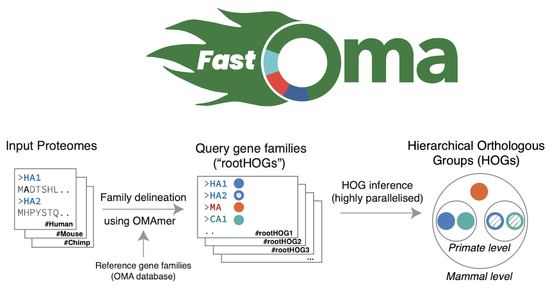
Figure 2. Overview of how FastOMA infers orthologs.
To the future!
As a community, we work collaboratively to advance the field and the lab has been contributing to the benchmarking datasets, making it possible to compare the performance of different tools, and ultimately advance the field. Earlier this year, in July, the Quest for Orthologs event (QFO8) was held at the University of Montreal, where recent advancements in orthology inference were discussed, and FastOMA was also presented there. The QFO 9 will be in Switzerland in 2026!
There are several directions for improving FastOMA’s accuracy and speed further. One exciting direction is taking advantage of recent advancements in protein structure prediction to reconstruct structural trees (Moi et al. 2023) in the context of orthology inference. This could really help boost resolution at deeper evolutionary levels. Besides, it would be very interesting to use gene order conservation, a.k.a, synteny information (Bernard et al. 2024), which could serve as an additional layer of information to refine orthology predictions. We hope our proposed hierarchical approach accompanied with several ideas will stimulate further developments.
So far, FastOMA has caught the attention of several labs around the world, who incorporated FastOMA in their studies. We are excited to hear how you plan to use FastOMA into your own research. Feel free to create a GitHub issue (https://github.com/DessimozLab/FastOMA) or send us an email if any help is needed!
To learn more see FastOMA academy: https://omabrowser.org/oma/academy/module/fastOMA
References
Altenhoff, Adrian M., et al. “OMA orthology in 2024: improved prokaryote coverage, ancestral and extant GO enrichment, a revamped synteny viewer and more in the OMA Ecosystem.” Nucleic Acids Research 52.D1 (2024): D513-D521. doi:10.1093/nar/gkad1020
Bernard, Charles, et al. “EdgeHOG: fine-grained ancestral gene order inference at tree-of-life scale.” bioRxiv (2024): 2024-08. https://doi.org/10.1101/2024.08.28.610045
Dessimoz, Christophe, et al. “OMA, a Comprehensive, Automated Project for the Identification of Orthologs from Complete Genome Data: Introduction and First Achievements” RECOMB 2005 Workshop on Comparative Genomics, LNCS 3678 (pp. 61-72). link
Emms, David M., and Steven Kelly. “OrthoFinder: phylogenetic orthology inference for comparative genomics.” Genome Biology 20 (2019): 1-14. doi:10.1186/s13059-019-1832-y
Fitch, Walter M. “Distinguishing homologous from analogous proteins.” Systematic zoology 19.2 (1970): 99-113. doi:10.2307/2412448
Majidian, Sina, et al. “Orthology inference at scale with FastOMA.” Nature Methods (2025) doi:10.1038/s41592-024-02552-8
Majidian, Sina, Mohammad Hossein Kahaei, and Dick de Ridder. “Minimum error correction-based haplotype assembly: Considerations for long read data.” PLOS ONE 15.6 (2020): e0234470. doi.org/10.1371/journal.pone.0234470
Moi, David, et al. “Structural phylogenetics unravels the evolutionary diversification of communication systems in gram-positive bacteria and their viruses.” BioRxiv (2023): 2023-09. doi:10.1101/2023.09.19.558401
Nicheperovich, Alina, et al. “OMAMO: orthology-based alternative model organism selection.” Bioinformatics 38.10 (2022): 2965-2966. doi:10.1093/bioinformatics/btac163
Tatusov, Roman L., et al. “The COG database: a tool for genome-scale analysis of protein functions and evolution.” Nucleic acids research 28.1 (2000): 33-36. doi:10.1093/nar/28.1.33
Train, Clément-Marie, et al. “Orthologous Matrix (OMA) algorithm 2.0: more robust to asymmetric evolutionary rates and more scalable hierarchical orthologous group inference.” Bioinformatics 33.14 (2017): i75-i82. doi:10.1093/bioinformatics/btx229
•
Author: Charles Bernard •
∞
For an evolutionary biologist, tracing today’s genomes back to key ancestors on the Tree of Life is a dream come true. With a collection of ancestral genomes, we could unravel the genetic steps that led to Life’s diversification from LUCA, the Last Universal Common Ancestor.
In practice, this means comparing modern genomes to find similar features—“orthologous” genes—passed down from common ancestors. By reversing this thinking, we can use these orthologous features as clues to “reconstruct” what ancestral genomes might have looked like.
But while much previous work has focused on reconstructing ancestral gene repertoires, reconstructing ancestral gene orders has been much more elusive.
In this post, I’ll dive into how we’ve developed a tool, EdgeHOG (1), to achieve this at a scale and speed never seen before (preprint here: https://www.biorxiv.org/content/10.1101/2024.08.28.610045v1).
Why do ancestral gene orders matter?
A genome isn’t just a random collection of genes; it has a structure that’s been shaped by evolution. Where a gene sits on a chromosome and its neighbours can matter a lot. Indeed, neighboring genes often work together (2). Plus, changes in gene order—genomic rearrangements—can lead to new traits and adaptations (3).
So, to understand the evolutionary history of these gene neighborhoods, we need to focus on gene adjacencies, not just the genes themselves. However, figuring out the gene order for every internal node on the Tree of Life is a huge computational challenge (4)…
How did we get into ancestral gene order inference?
When we wanted to analyze the link between gene function and gene adjacency across Life, we needed software that could reconstruct ancestral gene orders across the entire Tree of Life in one go, while accurately distinguishing between different copies of a gene in an ancestor.
But no tool could scale up to this level. Even the best tools, like AGORA (5) require reconstructing gene trees and perform pairwise comparisons of gene orders, which make them too slow to run on large datasets.
This is what drove us to create an algorithm with a clear goal: a linear time approach to reconstruct ancestral gene order, but without sacrificing accuracy.
How does EdgeHOG achieve linear-time complexity?
To infer ancestral gene orders at scale, our approach uses Hierarchical Orthologous Groups (HOGs). These model the lineage of genes from their ancestors to today’s species, assuming vertical inheritance.
By leveraging these gene lineages, our method uses “tree traversal” tricks to propagate or remove gene adjacencies along the species tree without any pairwise comparisons. Thanks to these tricks, our approach scales linearly with the size of the input phylogeny.
Since the software draws edges (gene adjacencies) between HOGs (proxies for ancestral genes), we called it EdgeHOG.
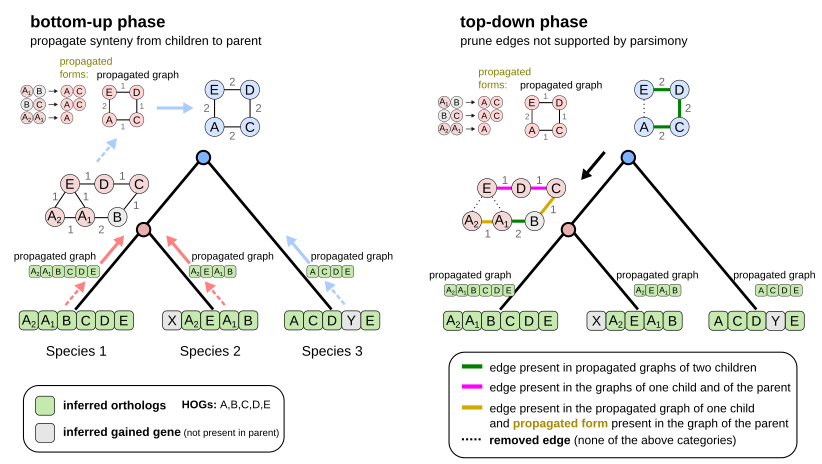
Here are the 2 first steps of EdgeHOG and the famous tree traversal tricks! The bottom-up phase propagates gene adjacencies up to the parental level of the species tree as long it is inferred by the HOG framework to have the two ancestral genes. The top-down phase essentially applies the Fitch algoritm and removes edges not supported by parsimony. Designing these tricks to comply with the constraint of linear time complexity was probably the most fun part of the project!
Fast and accurate
But EdgeHOG is not only fast, it is also very accurate! We validated it extensively on both simulated and real data. Across all benchmarks, EdgeHOG’s precision and recall met or exceeded the state of the art.
How to access EdgeHOG’s large scale inference of ancestral genomes?
The next step for us was to apply EdgeHOG to the entire OMA database, which currently includes 2,845 genomes from across the Tree of Life! This represent the first tree-of-life scale inference, resulting in 1133 ancestral genomes. You can explore these genomes on the OMA browser by clicking on Explore → Quick access to → Extant and ancestral genomes. For instance, check out the ancestral gene order for the last common ancestor of the mammals.
In the EdgeHOG paper, we also analysed the functions of the first ancestral contigs of genes ever reconstructed for LECA, the Last Eukaryotic Common Ancestor! These contigs contain genes that highlight core pathways like glycolysis, the pentose-phosphate shunt, amino-acid recycling, and histone organisation.
What kind of evolutionary analyses does EdgeHOG unlock?
In the lab, we’re using EdgeHOG to study the association between between gene order conservation and function conservation across different branches of the Tree of Life. We’re also dating gene adjacencies to identify old genomic neighbourhoods (like histone clusters in eukaryotes) or newer ones (like gene adjacencies on the sex chromosomes of animals).
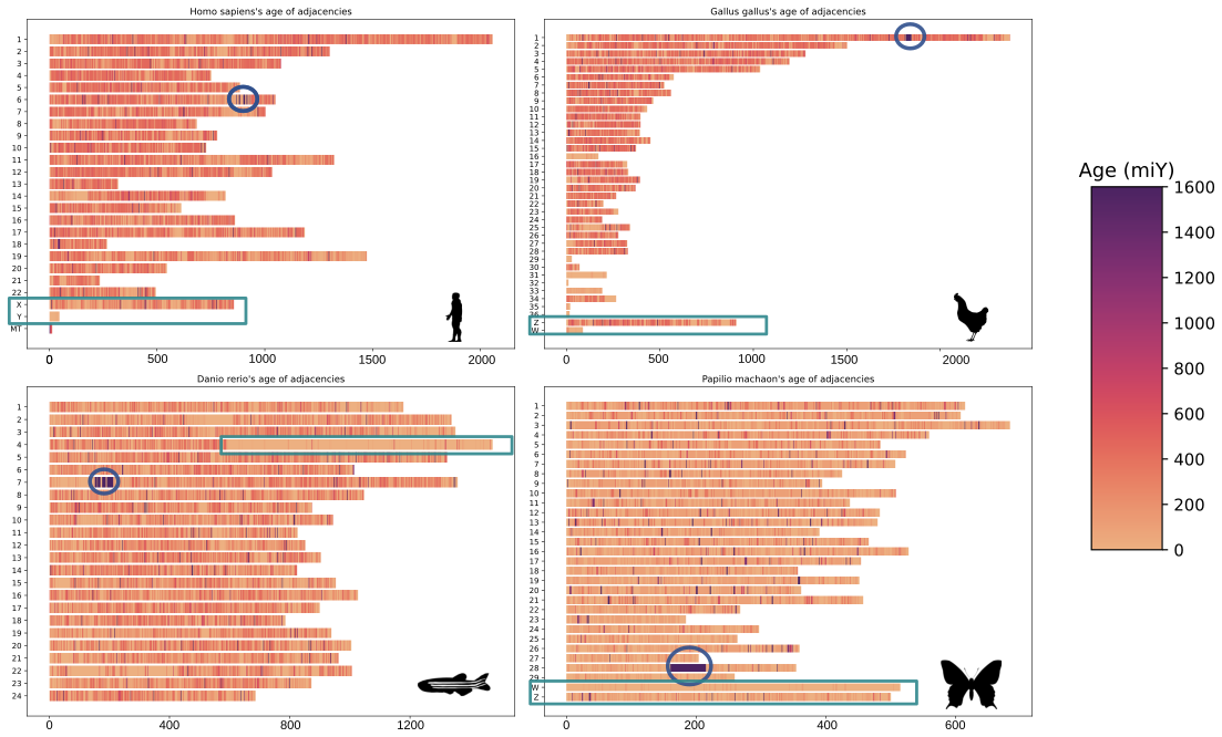
On these karyotypes, old histone clusters are circled in blue, and sex chromosomes are highlighted by rectangles. The estimated age of adjacencies is shown by the color scale on the right.
Overall, EdgeHOG opens up new possibilities in comparative genomics. For example, it helps track genomic rearrangements across a species tree, identify conserved gene clusters in clades of interest, or improve genome assembly by integrating gene order data from other species. Ultimately, knowing ancestral gene orders will enhance orthology inference by spotting highly divergent orthologs through their neighboring genes.
Do you want to try EdgeHOG on your datasets?
EdgeHOG is easy to use and available on GitHub https://github.com/DessimozLab/edgehog.
You’ll need a species tree, proteomes of each extant species (in Fasta files), and gene coordinates on contigs (in GFF files). Then, run our superfast FastOMA method to infer the HOGs. Finally, call EdgeHOG with the HOGs (OrthoXML file), the species tree (Newick file), and the path to the GFF files.
Now, you’re ready to perform big data ancestral gene order inferences, even with massive phylogenies of over 1,000 species! Try it on your favorite clade and let us know how it goes!
References
Bernard C, Nevers Y, Karampudi NBR, Gilbert KJ, Train C, Warwick Vesztrocy A, Glover N, Altenhoff A, Dessimoz C. EdgeHOG: fine-grained ancestral gene order inference at tree-of-life scale. bioRxiv 2024. https://doi.org/10.1101/2024.08.28.610045
Overbeek R, Fonstein M, D’Souza M, Pusch GD, Maltsev N. The use of gene clusters to infer functional coupling. Proc Natl Acad Sci U S A. 1999. https://doi.org/10.1073/pnas.96.6.2896
An X, Mao L, Wang Y, Xu Q, Liu X, Zhang S, Qiao Z, Li B, Li F, Kuang Z, Wan N, Liang X, Duan Q, Feng Z, Yang X, Liu S, Nevo E, Liu J, Storz JF, Li K. Genomic structural variation is associated with hypoxia adaptation in high-altitude zokors. Nat Ecol Evol. 2024. https://doi.org/10.1038/s41559-023-02275-7
El-Mabrouk N. Predicting the Evolution of Syntenies—An Algorithmic Review. Algorithms. 2021. https://doi.org/10.3390/a14050152
Muffato M, Louis A, Nguyen NTT, Lucas J, Berthelot C, Roest Crollius H. Reconstruction of hundreds of reference ancestral genomes across the eukaryotic kingdom. Nat Ecol Evol. 2023. https://doi.org/10.1038/s41559-022-01956-z
•
Author: David Moi •
∞
Breakthroughs don’t come every day, but the consequences of AlphaFold largely solving the 3D structure prediction problem has reshaped biology in profound ways. The sudden availability of protein structures for billions of proteins opens up many new possibilities. Last week’s two papers on the sequencing universe provide a compelling glimpse of the possibilities (here and here).
As someone who has been interested in tracing back the evolutionary origins of selected proteins—such as the cell fusion-mediating proteins fsx1 in plants, viruses, and archaea, or odorant receptors in insects—I have attempted to reconstruct phylogenies from structure in the past.
But I have faced two major issues:
Until AlphaFold came along, there typically wasn’t sufficient high-quality structure predictions as “starting material” to perform structure-based phylogenetics.
Even when I could obtain reasonably high confidence structures, the trees inferred from them were often met with skepticism—how reliable are these trees?
So now that high quality structure predictions are widely available, we could finally ask: are structures any good as starting material to infer trees? Specifically, how accurate are the reconstructed trees compared to sequences?
Today, we are super excited to report that structural phylogenetics works! What’s more, we found an approach that doesn’t just outperform traditional sequence-based methods for distant relationships; it also excels in resolving phylogenetic trees for closely related proteins. This post gives the gist of what we found—the full study is released as a preprint (1).
What’s the big deal with structural phylogenetics?
Before presenting our results, let’s take a step back. Why is structural phylogenetics potentially a big deal? Traditional phylogenetics, the study of evolutionary relationships among species or genes, has long relied on comparing the sequences of DNA, RNA, or proteins. While this approach has been immensely valuable, it does have its limitations. The primary challenge lies in the fact that the sequences of these biomolecules can change rapidly over time due to mutations and other factors, making it difficult to trace back their evolutionary history accurately when the divergence is very high. By contrast, proteins have unique three-dimensional structures that are intricately linked to their functions; these structures tend to change more slowly over evolutionary timescales compared to the sequences of the amino acids that make up the proteins since they are closely tied to the function of the protein.
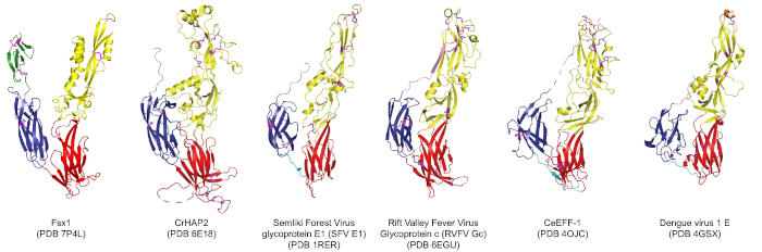
In this particular example close to my heart, we can see structural homology between functionally homologous proteins at wide evolutionary ranges. The examples shown span plants, metazoans, viruses and archaea. They share virtually no sequence homology. Ref: (2)
When we set out to do our work, however, we were not at all sure that it would work, let alone outperform sequence based methods. On the one hand, there have been decades of intensive tool and model refinements for sequence-based approaches, unlike its structure-based counterpart. But also, complications related to structure, such as allostery, flexible regions, and functional constraints could conceivably confound the evolutionary signal that can be extracted from structures.
Evidence that structure-based trees can outperform sequence-based trees
We tested a few structural approaches, and settled on an approach reconstructing distance trees using Foldseek’s “local structural alphabet” approach, which was developed in the lab of our collaborator Martin Steinegger to search for similar structures very rapidly—by encoding local structure motifs in a 20-letter alphabet and repurposing highly optimized alignment software originally developed to align amino acid sequences (3).
Testing and comparing the quality of phylogenetic trees empirically is tricky business. Most comparisons are based on simulated data, or by comparing the fit of data to different models. But how to compare trees that are reconstructed from entirely different kinds of input data? Luckily, our lab has accumulated quite some experience in these kinds of empirical observations, used previously to compare the accuracy of alignment (4 and 5) or orthology (6 and 7) methods. We used an approach which compares the propensity of inferred trees to recapitulate the known taxonomy of the species from which the proteins are sampled from.
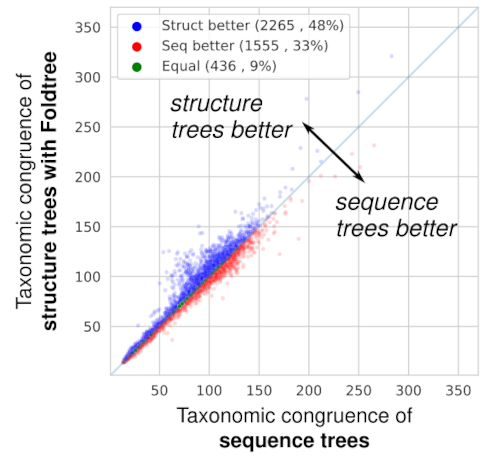
When comparing the taxonomic plausibility of thousands of trees derived from homologous protein families, Foldtree outperforms sequence-based phylogenetics. (In the paper, we show that after filtering the input set to families with high quality structures, the structural phylogenies perform even better!)
Amazingly, the trees we inferred in this way were more in line with the known taxonomy than those defined by sequence similarity! The input data can either be experimental crystal structures or AI structural models. Using good quality structures positively impacts the quality of the trees produced which means that as structural prediction methods get better, so will our structural trees.
The RRNPPA family: a first unifying phylogeny for peptidic quorum sensing proteins
To put our method to the test, we focused on a particularly complex gene family - the RRNPPA quorum sensing receptors (8). These receptors play a pivotal role in enabling communication and coordination among gram-positive bacteria, plasmids, and bacteriophages for crucial behaviors like sporulation, virulence, antibiotic resistance, conjugation, and phage lysis/lysogeny decisions.
The complex evolutionary pattern of this family is revealed in its name. Before AI structures, new homologs were previously only detectable after having been crystallized and each subfamily was added piecemeal to the overall picture, resulting in their particularly long acronym. As the family expanded researchers also attempted to piece together its evolutionary history, using a diverse set of methods, some of which relied on structural analysis. Using Foldtree we decoded the evolutionary diversification of these genes, shedding new light on their intricate history.
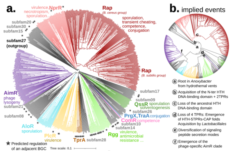
Compared to the sequence-based phylogeny, the Foldtree reconstruction of the RRNPPA family’s history is remarkably parsimonious. Several events such as domain architecture changes or transfers to the viral world appear only once in the tree.
Foldtree: infer a structural phylogeny for your favorite protein family

To make it easy to try this approach, as well as facilitate methodological improvements, we are releasing this new approach as an open source tool we call Foldtree. It’s available for download on GitHub (https://github.com/DessimozLab/fold_tree). Try it on your favorite protein family and let us know how it performs!
Exciting new research directions
High-accuracy structural phylogenetics has the potential to uncover deeper evolutionary relationships, elucidate unknown protein functions, and even refine the design of bioengineered molecules. The evolutionary histories of protein families in the viral domain, the start of eukaryotic life and the role of asgard archaea as well as the evolution of the prokaryotic mobilome are just a few cases where the fast pace of evolution has confounded sequence-based analyses and could be revisited. We believe this work represents an important step in investigating how structures are polished by the processes of evolution and how we can use this signal to peer further into the past than ever before.
References
Moi D, Bernard C, Steinegger M, Nevers Y, Langleib M, Dessimoz C. Structural phylogenetics unravels the evolutionary diversification of communication systems in gram-positive bacteria and their viruses. bioRxiv 2023.09.19.558401; doi: https://doi.org/10.1101/2023.09.19.558401
Moi D, Nishio S, Li X, Valansi C, Langleib M, Brukman NG, et al. Discovery of archaeal fusexins homologous to eukaryotic HAP2/GCS1 gamete fusion proteins. Nat Commun. 2022;13: 3880. doi:10.1038/s41467-022-31564-1
van Kempen M, Kim SS, Tumescheit C, Mirdita M, Lee J, Gilchrist CLM, et al. Fast and accurate protein structure search with Foldseek. Nat Biotechnol. 2023. doi:10.1038/s41587-023-01773-0
Tan G, Gil M, Löytynoja AP, Goldman N, Dessimoz C. Simple chained guide trees give poorer multiple sequence alignments than inferred trees in simulation and phylogenetic benchmarks. Proceedings of the National Academy of Sciences of the United States of America. 2015. pp. E99–100. doi:10.1073/pnas.1417526112
Dessimoz C, Gil M. Phylogenetic assessment of alignments reveals neglected tree signal in gaps. Genome Biol. 2010;11: R37. doi:10.1186/gb-2010-11-4-r37
Altenhoff AM, Dessimoz C. Phylogenetic and functional assessment of orthologs inference projects and methods. PLoS Comput Biol. 2009;5: e1000262. doi:10.1371/journal.pcbi.1000262
Altenhoff AM, Boeckmann B, Capella-Gutierrez S, Dalquen DA, DeLuca T, Forslund K, et al. Standardized benchmarking in the quest for orthologs. Nat Methods. 2016;13: 425–430. doi:10.1038/nmeth.3830
Bernard C, Li Y, Lopez P, Bapteste E. Large-scale identification of known and novel RRNPP quorum sensing systems by RRNPP_detector captures novel features of bacterial, plasmidic and viral co-evolution. Mol Biol Evol. 2023. doi:10.1093/molbev/msad062
•
Author: Yannis Nevers & Christophe Dessimoz •
∞
Proteins are fundamental to all life forms, dictating the complex biochemical interactions that maintain and drive the existence of every species. The functionality of a protein hinges on its structural domain organization, and the protein’s length is a direct manifestation of this. Given that every species has evolved under varying evolutionary pressures, one would intuitively expect protein length distribution to differ significantly across species.
Well, we report in a paper just published in Genome Biology that this is not the case.
Unexpected Homogeneity in Protein Length Distribution
In our study, we examined the protein length distribution across 2,326 species encompassing 1,688 bacteria, 153 archaea, and 485 eukaryotes. Counter to expectations, we observed a striking consistency in protein length distribution across these species. Though eukaryotic proteins were somewhat longer, the variation in protein length distribution was notably low compared to other genomic features such as genome size, gene length, number of proteins, GC content, and isoelectric points of proteins.
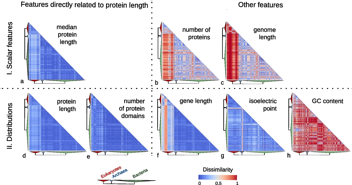
Features directly related to protein length are much more conserved than other features.
Exceptions: Errors or Biological Peculiarities?
We did note a few atypical cases of protein length distribution, but these were typically due to inaccuracies in gene annotation: no well-annotated model species displayed enrichment in small proteins, and those with a high number of small proteins were more likely to have incomplete or fragmented genome annotations.
Indeed, the outliers tended to include many more genomes scoring low in BUSCO quality score. The only exception we observed was the prevalence of longer proteins in the Ustilago fungal genus and the Apicomplexa phylum, known for their intracellular parasitic lifestyles.
This suggests that the actual variation in protein length distribution might be even smaller than what we reported. Hopefully, resequencing and reannotation efforts will help solve this issue in the future: we already noticed a few species getting updated proteomes where the length distributions gets more similar to the typical one!
A Universal Selection Force at Play
The startling uniformity of protein length distribution across diverse species suggests a strong, universal selective pressure, maintaining a high proportion of the coding sequence within a specific length range. In the discussion part of the paper, we articulate a number of potential explanations, but these remain highly speculative.
More positively put, the evolutionary forces behind the uniformity of protein distribution and their potential impact on fitness remain exciting areas of exploration!
Protein Length Distribution: A New Criterion for Gene Quality?
This observation led us to propose the use of protein length distribution as a new criterion of protein-coding gene quality upon publication. Considering that the overabundance of spurious proteins could potentially bias downstream analyses, this quality measure could aid in identifying and rectifying annotation errors. We also encourage everyone to take a look at this simple criterion when selecting proteomes for comparative genomics analysis.
Story behind the paper
The basic premise of the paper, exploring protein length distribution across the tree of life, may seem straightforward at first glance. Not quite. It started as part of Yannis’s PhD in Odile Lecompte’s lab in Strasbourg—and a few questions: what are the characteristics of the thousands of publicly available proteomes? How to decide which to include in large scale analyses? It took another three years of Yannis’s postdoc, with about half of that time spent in the peer-review process.
Perhaps the most revealing testament to the depth of this work is the supplementary PDF, a 68-page document filled with detailed data and analyses. Moreover, anyone interested in the peer-review history of our paper can delve into the 18-page record available here.
The journey is the reward, they say; well in this instance, we are quite happy to have reached our destination!
Reference:
Nevers, Y., Glover, N.M., Dessimoz, C, Lecompte, O. Protein length distribution is remarkably uniform across the tree of life. Genome Biol 24, 135 (2023). https://doi.org/10.1186/s13059-023-02973-2
•
Author: Christophe Dessimoz & Fritz Sedlazeck •
∞
We just published a method to build phylogenetic trees directly from raw reads, bypassing time-consuming steps such as genome assembly. This post gives the short story and the backstory. In particular, find out below what Read2Tree has in common with “Smoke on the Water” from the band Deep Purple.
In biology, phylogenetic trees are everywhere. They help us understand the relationships between species, genes, or cells—how they evolved, and how they’re related.
The sequencing revolution provides the raw material to infer phylogenetic trees, but building state-of-the-art phylogenetic trees requires tedious steps from read curation, de novo assembly, gene annotation, ortholog identification to tree inference, which can take many months to run—millions of CPU hours invested in this process are not uncommon—and specialised knowledge to oversee this process.
That’s where Read2Tree comes in. Our new approach to tree inference bypasses the usual steps of genome assembly, annotation, and orthology inference. Instead, it uses existing knowledge of the protein sequence universe to directly reconstruct comprehensive sequence alignments from raw sequencing reads.
The approach is vastly faster than traditional methods and in many cases more accurate—the exception being when sequencing coverage is high and reference species very distant. Read2Tree is also flexible, working with genome and transcriptome, short and long reads, and sequencing coverage as low as 0.1x.
We were encouraged by the buzz the Read2Tree manuscript elicited on bioRxiv last year, and are delighted it has now been published in Nature Biotechnology.
What is Read2Tree good for?
A nice illustration of Read2Tree’s potential was the reconstruction of a phylogeny of coronaviruses, which processed on the same tree diverse Coronaviridae sequences as well as 10,000 raw SARS-CoV-2 datasets from the Short Read Archive. The reconstructed tree was consistent with the lineage classification obtained from the UniProt reference proteomes, accurately recovering the main coronavirus genera and all subgenera (Figure 1). At the same time, the same phylogeny accurately clustered the sequences according to CDC variants of concerns classification. These results demonstrate the versatility and scalability of Read2Tree, making it suitable for both zoonotic surveillance and human epidemiology.
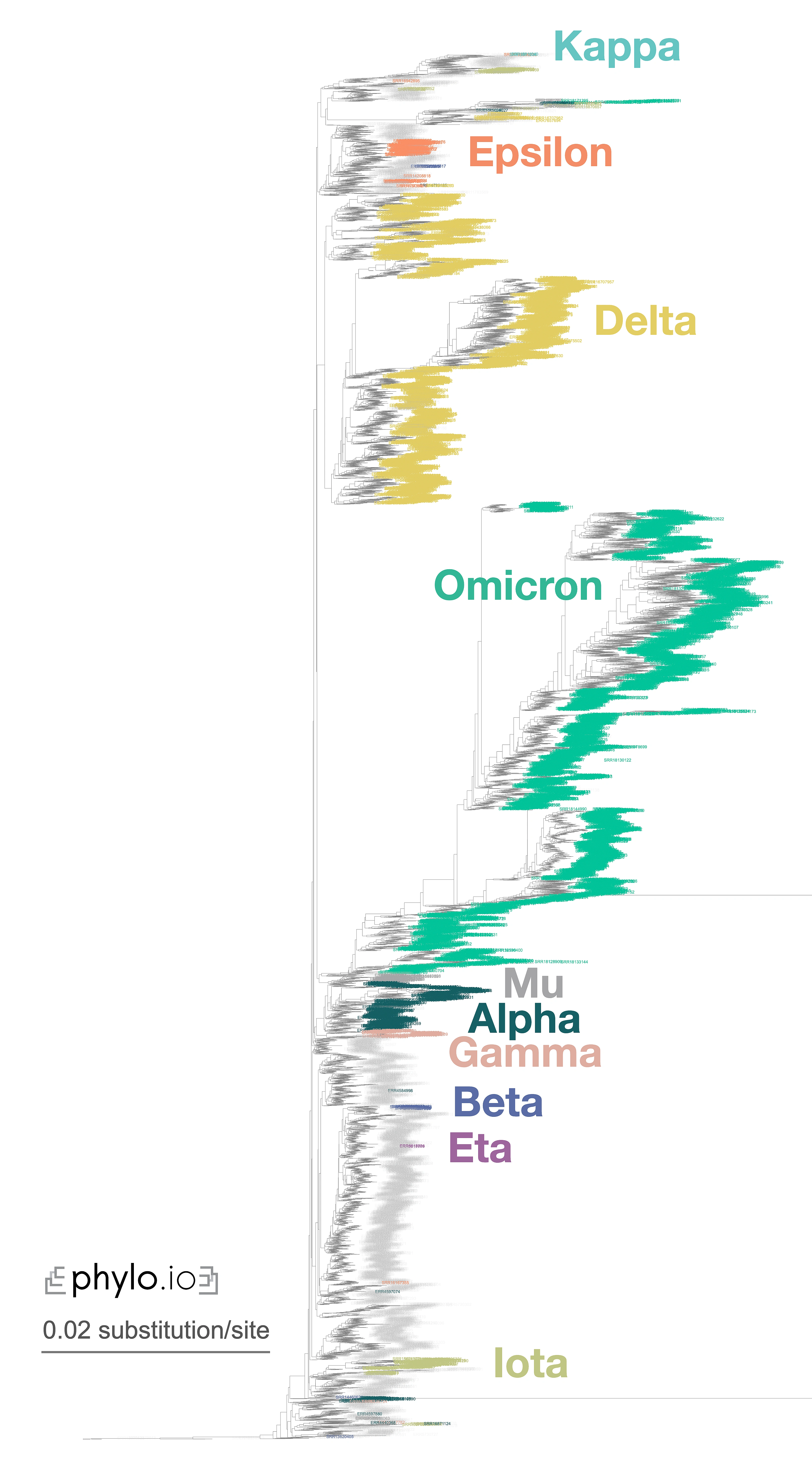
Figure 1—Zoomed-in display of a tree inferred using Read2Tree on 10,283 samples whole genome SARS-CoV-2 samples. Classification in colour was obtained from [https://harvestvariants.info](https://harvestvariants.info), where grey leaves are unclassified according to the CDC label. The colour clustering shows that the Read2Tree-based tree recovers consistent classification. Click on the tree to see it full screen.
The ability to reconstruct phylogenetic trees from raw reads has additional advantages. Some genomes are deposited with poor or even entirely absent protein annotation sets. Processing genomes directly from raw reads can avoid this limitation and also decrease biases that arise from relying too heavily on specific reference genomes. Although some efforts have been made to “dehumanize” non-human great ape genomes, other clades still face similar biases that can be significantly reduced by processing raw reads.
Who might find it useful?
We think Read2Tree will be especially useful for small labs with limited bioinformatics expertise and computational resources, allowing them to perform state-of-the-art phylogenomics on particular species or environments of interest.
But it’s not just small labs that can benefit from Read2Tree. Large consortia can also use it to regularly update their trees as new genomes are sequenced. This is especially important as more and more projects around comparative genomics are underway, such as the Earth BioGenome, the Darwin Tree of Life, or the European Reference Genome Atlas projects.
In addition, Read2Tree’s ability to infer trees from much lower coverage than traditional methods means it can also be useful for quality control early in the process. This makes it a valuable tool for environmental and metagenomic applications, especially when combined with genome binning techniques.
Overall, Read2Tree is a powerful method for inferring phylogenetic trees directly from raw sequencing reads. We hope it will help make phylogenetic tree inference faster, more accurate, and more accessible to a wider range of researchers.
What’s next?
Now that the introductory Read2Tree paper is published, we are excited to explore new potential applications that we haven’t been able to tackle so far. For instance, we have already received inquiries from researchers interested in using Read2Tree for ancient DNA applications or for monitoring systems that require fast turnaround time and low coverage.
Moving forward, we have two main goals. First, we aim to expand Read2Tree’s capabilities to handle multi-species samples, which will enable an even broader range of applications in the metagenomics field. While long-read applications may offer the most benefit, we are confident that Read2Tree’s ability to perform well with short-reads will also prove valuable in detangling multiple species.
Secondly, we plan to explore the use of Read2Tree in single-cell sequencing. This rapidly growing field involves sequencing individual cells, including cancer cells, and analysing their genetic information. Given Read2Tree’s ability to operate with low coverage levels (down to 0.2x), we believe it could facilitate fast and accurate characterization of tumour or cell evolution.
We hope that Read2Tree will help streamline and democratise comparative genomics analyses. We are excited to see how researchers will apply this tool to further advance our understanding of genetics and evolution.
What’s the backstory?
Both of our labs (Fritz Sedlazeck’s and Christophe Dessimoz’s) have been collaborating for many years, and we’ve always enjoyed exchanging ideas even though our research interests are quite diverse. One of our interests over the years is how to combine our expertise in sequence analysis and ortholog comparison to develop new methodologies and gain new insights into biology.
It was during one of Fritz’s visits to Christophe’s lab in Lausanne, Switzerland, that we started brainstorming ideas for a project that led to Read2Tree. Our goal was to overcome the limitations and bottlenecks of comparative genomics. We had some amazing cheese risotto, and the beautiful scenery fueled our discussions further (Figure 2).

Figure 2 — Fritz alleges that the epiphany of Read2Tree took place with this view from his hotel room in Montreux, Switzerland, during a collaborative visit to Christophe’s group. It’s not entirely implausible, considering this very view [inspired the song “Smoke on the Water” by Deep Purple](https://en.wikipedia.org/wiki/Smoke_on_the_Water#History).
David Dylus, the first author, was convinced that it was possible to bring our ideas to life, although he did not anticipate how much time and effort it would take (Figure 3). Even after he moved on to a new role in the pharmaceutical industry, he continued to work on Read2Tree after regular work hours. And when the COVID-19 pandemic hit, we had to face additional challenges, such as maintaining regular meetings and pushing the manuscript forward while not compromising on quality. We also faced technical issues, such as hard disk crashes and cluster updates that led to data loss, but David hang on.
Completing the paper was not an easy task, and one of the biggest challenges was organising and identifying all of the SRA data sets, including those related to yeast and COVID-19. Despite these challenges, we were able to bring the project to completion. It was a special joy to present the work at ISMB 2022, where Fritz and Christophe had the wonderful opportunity to meet in person, and we continued to discuss our work while enjoying good food and drinks by beautiful Mendota lake in Madison, Wisconsin.
In summary, nice food and lakeside views were instrumental in the making of Read2Tree.
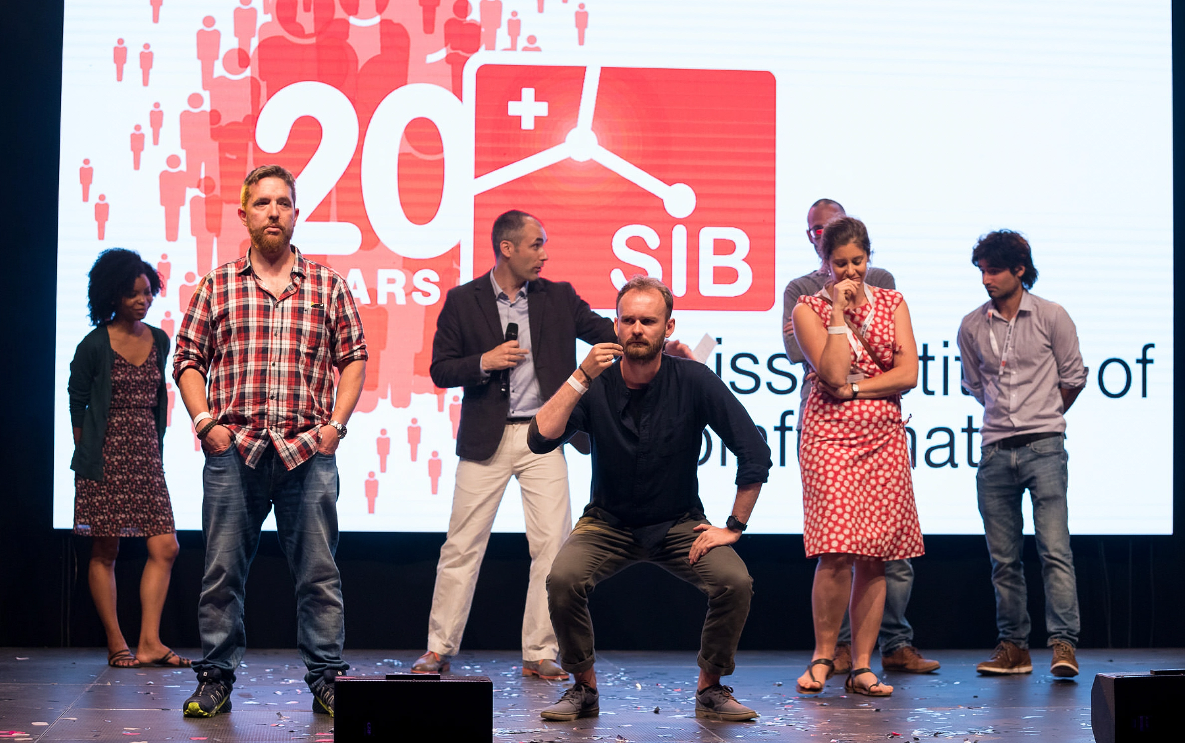
Figure 3 — First author David Dylus performing on stage (centre, crouching) on the occasion of SIB Swiss Institute of Bioinformatics’s 20th anniversary—a period of rapid progress in the development of Read2Tree. Though no-one is entirely certain, rumour has it that David is miming “sipping a cup of tea while looking into the distance”, in line with our theme of sustenance, inspiring landscapes, and scientific progress.
Note this blog post was first published on the Nature Communities blog here.
Reference
Dylus, D., Altenhoff, A., Majidian, S. et al. Inference of phylogenetic trees directly from raw sequencing reads using Read2Tree. Nat Biotechnol (2023). doi:10.1038/s41587-023-01753-4.
•
Author: Yannis Nevers •
∞
I am excited to introduce our preprint for our new tool OMArk. We hope our software will help fill a gap in assessing the quality of gene annotation sets.
Many studies directly rely on the protein-coding gene repertoires (“proteomes”) predicted from genome assemblies to perform their comparisons. Doing so, they rely on the assumption that the predicted gene content of all genomes are of homogeneous quality and an accurate reflection of reality. Yet in practice, this assumption is rarely met, with protein-coding genes often missing or fragmented in the reported proteomes, non-coding sequences wrongly annotated as coding genes by gene predictors, or contamination from other species wrongly included among the reported sequences.
Why a new proteome quality tool?
Our new method, OMArk, provides a way to easily and comprehensively measure different aspects of proteome quality: completeness of the gene repertoire, consistency of the included genes at the taxonomic level, whether they have doubtful gene structures, and presence or not of inter or intra-domain contamination. Furthermore, contrary to existing methods, OMArk does not rely on a manual selection of reference dataset; instead, it automatically identifies the most likely taxonomic classification of the test proteomes. It can thus process any test proteome across the tree of life using a universal reference database.
Conceptual overview of OMArk (left) and how the innovative consistency assessment is computed (right).
OMArk is accurate and provides new insights
We performed extensive validation of the method by introducing controlled amounts of noise, fragmentation and contamination to reference proteomes and accurately estimating these amounts using OMArk. We also performed a large-scale analysis of 1805 eukaryotic UniProt Reference Proteomes with our software and were able to detect unambiguous cases of quality issues, either caused from incompleteness, contamination, or inclusion of translated non-coding sequences. In the most extreme case, we found a plant proteome with contamination from eight different species—fungi and bacteria.
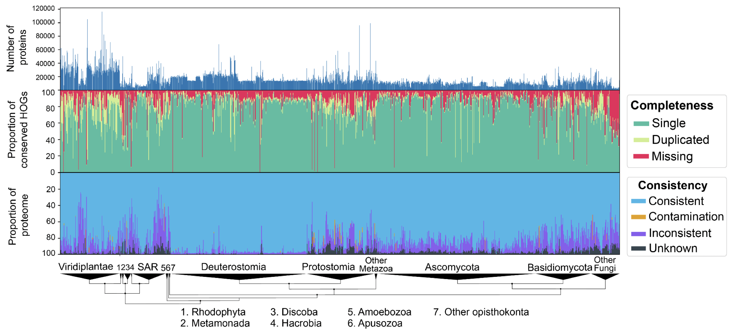
OMArk results on 1805 Eukaryotic proteomes from UniProt. Interactively check results on the OMArk webserver, e.g. for the current cowpea weevil reference proteome.
Why does the consistency metric matter? For example, comparing the Ensembl gene set for two assemblies of Bombus impatiens. We can detect a major improvement in consistency (including contamination removal) for a similar completeness.
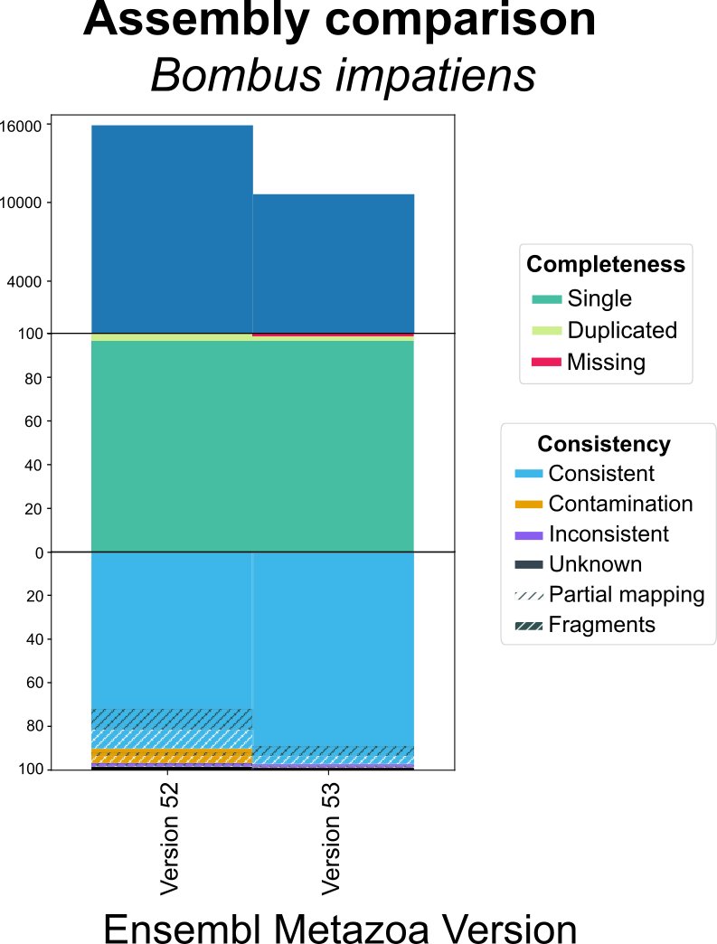
OMArk can reveal improvements in genome assemblies/annotations even if completeness has not substantially changed.
OMArk is quick and easy to run
OMArk can be easily used as a command line tool or on our OMArk webserver. On the webserver, you can submit a FASTA file of your proteome and get results in about 30 minutes. Nothing more required. You can visualize the results and directly compare it to precomputed results from closely related species (UniProt reference proteomes).
More details can be found in the preprint linked below. Please let us know how the tool works for you!
Reference
Yannis Nevers, Alex Warwick Vesztrocy, Victor Rossier, Clément-Marie Train, Adrian Altenhoff, Christophe Dessimoz, Natasha M Glover
Quality assessment of gene repertoire annotations with OMArk
Nature Biotechnology 2024 doi:10.1038/s41587-024-02147-w
•
Author: Charles Bernard •
∞
This year, the MCEB international conference was held in Switzerland for the first time in its history.
During five days, from June 26th to 30th 2022, experts in mathematical and computational evolutionary biology
from all over the world exchanged about their passion in Chateau d’Oex,
in the heart of the welcoming mountains of the regional natural park of Gruyeres.
Here is a little summary on this annual not-to-be-missed event for evolutionary biology aficinionados.
The edition 2022 of the international MCEB conference brought together a hundreds of scientists
from diverse disciplines and at different stages of their career,
from PhD students to world-renown senior scientists.
During five consecutive days, the Chateau d’Oex has hence been the improbable scene of inspiring exchanges
about evolution between mathematicians, computational biologists, evolutionary biologists, ecologists,
epidemiologists and cancer biologists.
View from the conference venue (left) and cheese making social activity (right).
In total, 6 one-hour talks and 20 short talks were given to present
epistemological perspectives, recent methodological advances and challenges yet to be addressed
for reconstructing the evolutionary history of the genes, genomes, populations and species
observed then and today on Earth.
As a mirror of the truly interdisciplinary nature of the event, a wide range of phylogenetic structures
have been discussed during these five days.
Networks of gene flows, phylogenetic trees, or genealogical trees predicted by coalescent theory
were on the menu of this year.
Experts specialized in introgressive events such as horizontal gene transfers or endosymbioses
provided insights on the methods and challenges to model reticulate evolution.
With this respect, an inspirational talk was given on how ghost lineages that went extinct in the past
but nonetheless exchanged some DNA with ancestors of extant species could mislead our interpretation
of the directionality of gene flows within phylogenetic networks.
Lectures on the theoretical advances that were made throughout the last 50 years in the reconstruction
of gene and species phylogenetic trees were then given by world leaders in the field of phylogeny.
In particular, they provided mathematical evidence that contrary to what is practiced today
to reconstruct species trees, neither the consensus tree of several gene trees
nor the tree inferred from the concatenated alignment of these genes
actually give a good approximation of the phylogeny of the different species encoding these genes,
which highlights the urgent need to pursue methodological efforts to better model species evolution.
On shorter evolutionary timescales, numerous mathematical models to infer geneological trees
of human populations or cancer cell lineages were also presented during the conference.
Poster session (left) and group photo (right).
Finally, a strong focus was placed this year on methods for coupling phylogenetic inferences with phenotypical,
ecological, archaeological, geographical, epidemiological and medical data in order to study
how traits or diseases evolved across space and time.
Striking examples of these integrative analyses were provided by methodologies to retrace with accuracy the evolution
of the recent Sars-Cov2 and MERS-Cov pandemics over time and space.
In addition to these talks of exceptional scientific quality, two poster sessions animated
by junior researchers and students took place during the conference and were truly appreciated
by every participants for the scientific excellence of the posters and the conviviality of the moments.
Overall, through five days of scientific presentations, poster sessions, dinners, parties
and social activities such as hiking in the Alpes or visiting a cheese factory,
scientific exchanges and informal talks were fostered and allowed to create news bonds within this community of researchers.
The MCEB 2022 conference was a great success as it enabled a diversity of scientists from all over the world to meet,
exchange on their work and build new collaborations!
•
Author: Natasha Glover •
∞
I recently became aware of the memes and popular science articles going around the internet claiming that we share 50% of our DNA with bananas. For example:
Source: http://www.quickmeme.com/meme/36gnaz
I work in the Dessimoz lab at the University of Lausanne, and here we are in the business of comparing genes. In fact, I’ve had a similar question before一 what percentage of our protein-coding genes do we share with another plant, Arabidopsis thaliana. I computed the number as being closer to 17%.
I wanted to get to the bottom of this question once and for all: What percentage of a human’s “genetic material” is shared with a banana? There have been several other blog posts from scientists touching on this question (Neil Saunders: “50% bananas”, Stack Exchange skeptics: “Do humans share 50% of their DNA with bananas?”, Sanogenetics: “Are We Genetically Similar To Bananas And Why Is This Important For Research In Disease?”).
However, I wanted to go a little deeper into:
- Where this number came from, and the extent of it being spread on the internet.
- What exactly do we mean by “shared genetic material”?
- Some results I computed in attempts to put this controversy to rest once and for all.
In this blog post I will attempt to address these questions.
Where did the mythical 50% come from anyway?
After performing a quick google search, it seems that the relatedness between a human and a banana has been a popular question. With a cursory, non-exhaustive search, I show in the table below eight sources who report that 44-60% of the human genome is “shared” with banana.
| Source |
quote |
| Irishnews.com |
“But we are also genetically related to bananas – with whom we share 50% of our DNA – and slugs – with whom we share 70% of our DNA.” |
| getscience.com |
“Banana: more than 60 percent identical. Many of the “housekeeping” genes that are necessary for basic cellular function, such as for replicating DNA, controlling the cell cycle, and helping cells divide are shared between many plants (including bananas) and animals.” |
| thenakedscientists.com |
“So where does this banana statistic come from? Is it just complete nonsense? Well, no. We do in fact share about 50% of our genes with plants – including bananas.” |
| PopSci.com |
“Bananas have 44.1% of genetic makeup in common with humans.” |
| MythBusters (tv show) facebook |
“#sciencefact: Humans share approximately 98% of their DNA with chimps, 70% with slugs, and 50% with bananas! http://bit.ly/qsWX8p” |
| mirror.co.uk |
“Humans share 50% of our DNA with a banana.” |
| Business Insider |
“The genetic similarity between a human and a banana is 60%.” Source: National Human Genome Research Institute (However, no link and when I tried to search) |
| Sundaypost.com |
“Yes, and we share 50% with bananas. It’s not surprising, if you look at the basic mechanism of biochemistry.” |
What is disconcerting is that at least half of these sources come from popular science websites or science sections of newspapers, yet few have any sort of citation at all. The only exceptions were Popular Science, which gave DataScope as a source, and Business Insider, who cites the National Human Genome Research Institute. However, neither of these articles give a link or further information to follow up on.
Upon further digging, I found one recent article published on howstuffworks entitled “Do People and Bananas Really Share 50 Percent of the Same DNA?”, which contains an interview with one of the scientists from the Human Genome Research Institute, where he explains how they arrived at that number.
“Brody says the experiment was not published, as most scientific research is. Instead, it was generated to be included as part of an educational Smithsonian Museum of Natural History video called ‘The Animated Genome.’ That video noted that DNA between a human and a banana is ‘41 percent similar.’””
The article goes on to explain that this 41% figure comes from a blast search between protein sequences of human and banana. They found about 7,000 hits, and the average percent identity of these hits was 41%. He goes on to note:
“This is the average similarity between proteins (gene products), not genes… Of course, there are many, many genes in our genome that do not have a recognizable counterpart in the banana genome and vice versa.”
So when we get to the bottom of it, the 50% figure is actually 40% average amino acid percent identity between 7000 blast hits of human and banana.
What do we mean when we say “we share 50% of our DNA with a banana”?
All living organisms descended from a common ancestor, and therefore all living organisms have some genes in common. What determines how many genes in common depends on how far back in time the two species shared a common ancestor. For example, humans and chimps share such a high percentage of genes, because we only diverged ~6 MYA1. However, human and banana (more specifically the common ancestors which led to human and banana) split around 1.5 BILLION years ago2. Talk about a banana split! Therefore we would expect a lot less to be conserved.
As brought up by Neil Saunders in his blog post, “What does ‘we share 50% of our DNA’ really mean?” A non-biologist perhaps might not see the nuance in this question. If I were going to play the devil’s advocate, I could say that a child shares 50% of its DNA with their parents. Or even that every organism shares 100% DNA, as it is all made up of Gs, Cs, As, and Ts. Thus, it is important to be specific on what we’re talking about.
This shared DNA could be referring to a number of things: protein-coding genes, non-coding genes, transposable elements, the percent that gets aligned in a whole genome alignment3, etc. Each of these specific features evolve at different rates, and thus will be more or less conserved between any given species.
Well, how do we know if these genomic features are conserved?
Generally, sequences are compared by making an alignment, and then computing the percent identity or evolutionary distance between the two sequences. If the sequences are sufficiently similar, they can be declared as conserved. Thus, “conserved” can be seen as either categorical (i.e. conserved or not), and then specified as a quantitative value (conserved to a certain degree). For more information, see the Wiki page on conserved sequences.
What are the genomic features the most likely to be conserved?
“Conservation indicates that a sequence has been maintained by natural selection” (wiki). Genes, or DNA sequences, encode for the proteins. Proteins are slower to evolve and change than the DNA, due to the redundancy of the genetic code. Thus proteins are the genomic feature most likely to be conserved between evolutionary distant species. While it is true that other genomic features such as non-coding regulatory sequences or non-coding RNA can be conserved over long evolutionary distances, they are far more likely to diverge in sequence than proteins4,5. Other genetic features such as transposable elements, or intergenic “junk DNA” are even less likely to be conserved, as their sequences are under less selection pressure and accumulate mutations at an even higher rate.
It is important to note that while we generally declare sequences to be conserved on the basis of sequence similarity, sequences may be still conserved and lack similarity. For example, two sequences might be conserved in the structure of the protein, indicating homology 6,7. Additionally, sequences might be in a syntenic position, indicating ancestral conservation, but may also lack sequence similarity 8. Thus, it is possible for some genes to be shared between evolutionary distant species, but they may fly under the radar of our current homology-inference tools. So, in order to investigate the 50% shared DNA claim, we can only focus on sequence conservation which we are able to detect.
To understand how much of the genome is conserved between banana and human, I will look at proteins because it’s the feature most likely to be conserved between human and banana. This is to be as permissive as possible in attempts to give the benefit of the doubt to the 50% meme.
Now the question is, how do we compare all the proteins in one species to all the proteins in another species and see which ones “match”, i.e. descended from a common ancestral gene? This is a fundamental problem important for studying evolution. Orthologs are the term we use for genes in different species that started diverging due to a speciation event, i.e. “corresponding” genes between species. This is where our lab’s expertise comes in: we maintain Orthologous Matrix, which is a method and database for finding orthologs between many species.
Orthologs in common between human and banana
I wanted to see what percent of human’s genes are orthologous to banana genes一and vice versa一what percent of banana’s genes are orthologous to human’s. To compare several different methods, I tested three common methods for finding orthologs: OMA9, OrthoInspector10, and best-bidirectional hit (using BLASTP)11. For each method, I divided the number of orthologs found by the number genes in the genome to come up with a percentage of each genome that is shared. You can find all the details here jupyter notebook, but the results are summed up in the graph below:
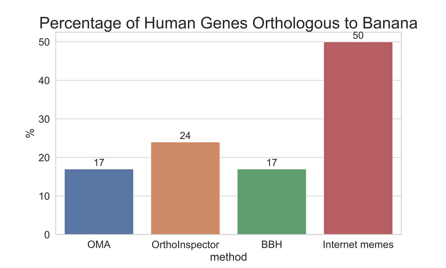
Comparison of ortholog methods
As you can see, all the orthology-inference methods tested show a maximum of 25% of human genes to be orthologous to banana. Again, these results give the most leeway, as we used protein sequences, which are the genomic elements the most likely to be conserved.
Additionally, I investigated the percentage of a whole-genome alignment that would be shared between banana and human. Since this is computationally intensive, I used Ensembl Compara, which has precomputed pairwise whole-genome alignments between a number of species. A whole-genome alignment looks at the whole genome, not just genes, as well as compares DNA rather than proteins. They didn’t have results between human and banana, but here are the results between human and chimp, mouse, and zebrafish:
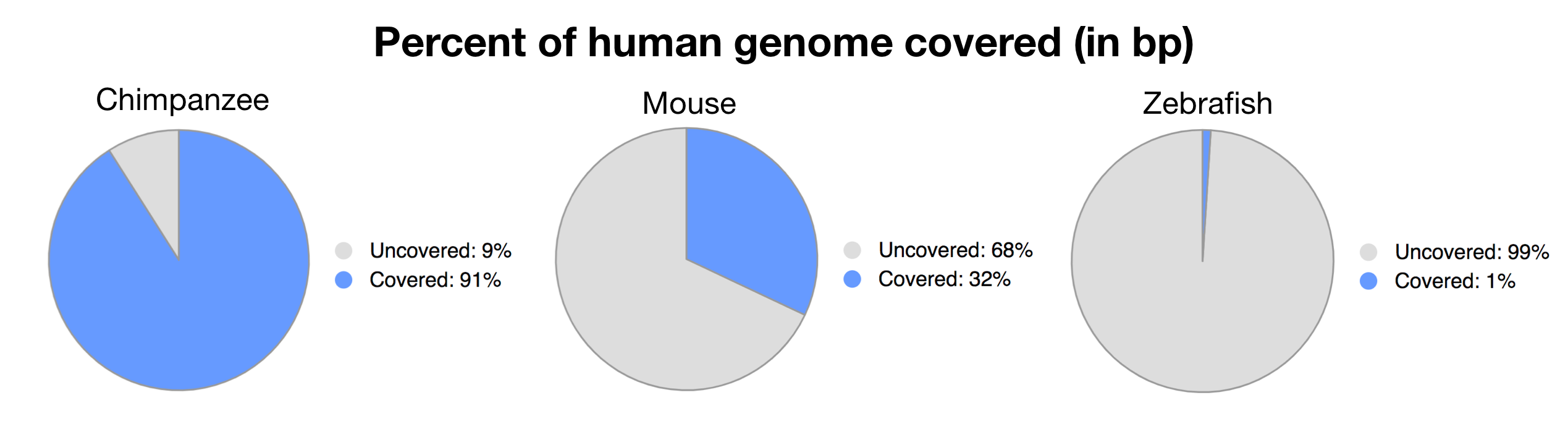
Data obtained from https://uswest.ensembl.org/info/genome/compara/analyses.html#
As we get progressively further in evolutionary distance, we get a smaller and smaller percentage of the genome which is able to be aligned. We can presume that plants would be even less than 1%, a far cry from the 50% as reported by internet memes.
So whichever way you slice it, humans share at most ¼, not ½ of its genetic material with banana (at least what we are able to detect)!
What do these human-banana orthologs DO?
Now that we have found the human-banana orthologs, we can try to gain some insight into what these genes do. To do this, I performed a Gene Ontology (GO) enrichment analysis of the human genes. GO enrichment works by assigning functional annotations to all of the sequences, then looking for a statistical overrepresentation of certain functions in a subset of genes compared to the entire genome.
I used the PANTHER Overrepresentation Test web server for the GO enrichment, then used GO-Figure12 for summarizing and visualizing the most enriched Biological Processes. All the details are in the jupyter notebook.
The top 10 overrepresented GO terms, i.e. a summary of the most common functions of the human genes with orthologs, is shown below:
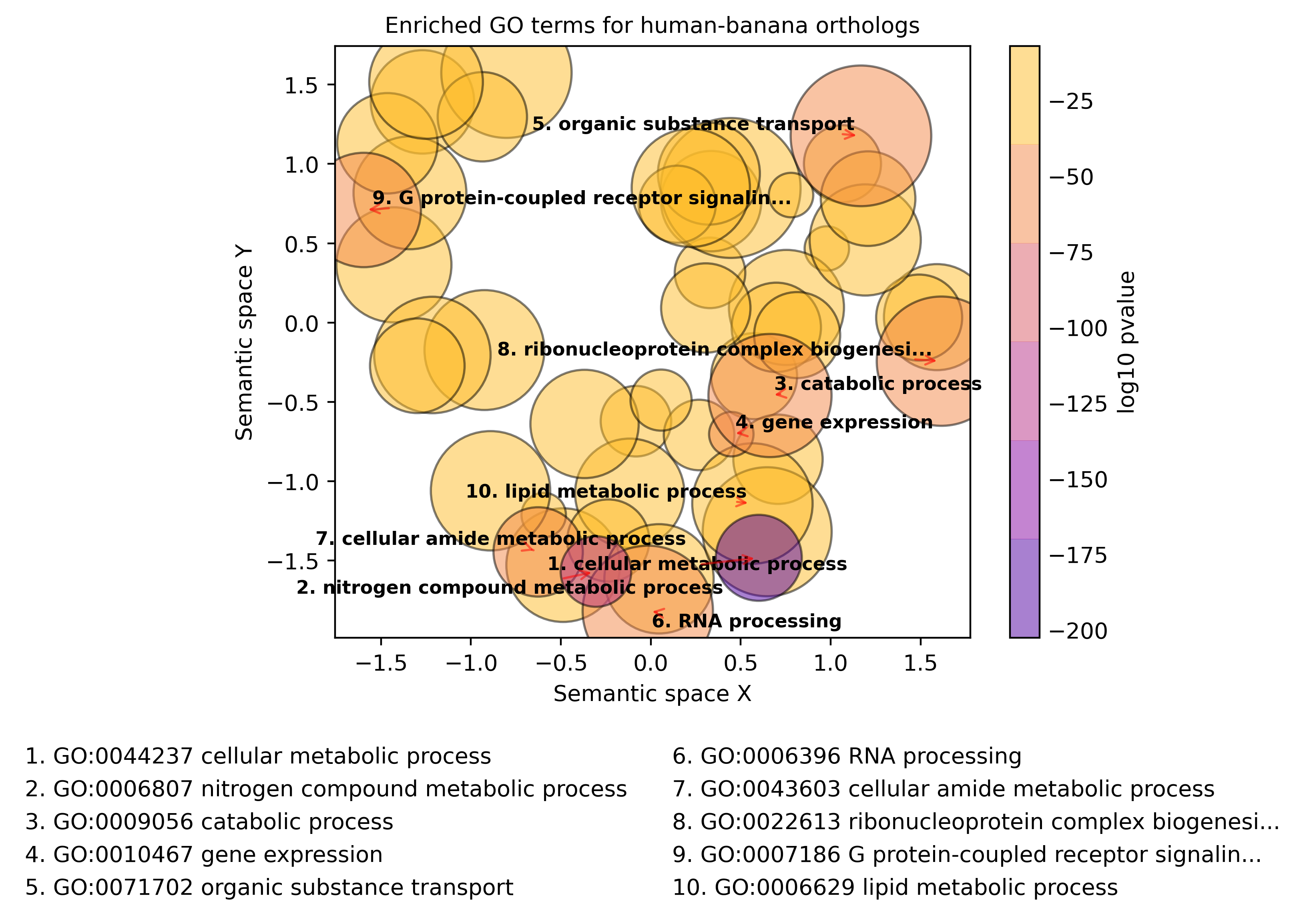
Top 10 overrepresented GO Biological Processes for human protein-coding genes with banana orthologs
We can see that the human-banana orthologs are highly enriched for basic, metabolic processes such as “cellular metabolic process,” “gene expression,” and “RNA processing.” These biological functions are likely genes which encode for cellular processes that are essential for eukaryotic life!
Take home message
- “Humans share 50% of DNA with banana” is a statement that has very little meaning.
- We must be careful to be precise in our language. We have to clarify what we mean when we give a percentage of “shared genetic material/DNA/genome.” I argue that the percentage of protein-coding genes is currently the best way to compare evolutionarily distant species
- There’s no evidence that humans have 50% of detectable orthologs with a banana. In my analysis, I show between 17 and 24%, depending on which method was used. As scientists, we have to do a better job communicating science with each other and with the general public.
Even though we don’t have 50% genes in common with banana, we still have ~20% which is nothing to scoff at! The functions of these genes are most likely basic housekeeping proteins involved in metabolic processes that are necessary for most, if not all of eukaryotic life. It is amazing that these genes have been conserved over 1.5 billion years of evolution!
References
- Patterson, N., Richter, D. J., Gnerre, S., Lander, E. S. & Reich, D. Genetic evidence for complex speciation of humans and chimpanzees. Nature 441, 1103–1108 (2006).
- Wang, D. Y., Kumar, S. & Hedges, S. B. Divergence time estimates for the early history of animal phyla and the origin of plants, animals and fungi. Proc. Biol. Sci. 266, 163–171 (1999).
- Armstrong, J., Fiddes, I. T., Diekhans, M. & Paten, B. Whole-Genome Alignment and Comparative Annotation. Annu Rev Anim Biosci 7, 41–64 (2019).
- Ransohoff, J. D., Wei, Y. & Khavari, P. A. The functions and unique features of long intergenic non-coding RNA. Nat. Rev. Mol. Cell Biol. 19, 143–157 (2018).
- Diederichs, S. The four dimensions of noncoding RNA conservation. Trends Genet. 30, 121–123 (2014).
- Illergård, K., Ardell, D. H. & Elofsson, A. Structure is three to ten times more conserved than sequence—a study of structural response in protein cores. Proteins 77, 499–508 (2009).
- Zheng, W. et al. Detecting distant-homology protein structures by aligning deep neural-network based contact maps. PLoS Comput. Biol. 15, e1007411 (2019).
- Vakirlis, N., Carvunis, A.-R. & McLysaght, A. Synteny-based analyses indicate that sequence divergence is not the main source of orphan genes. Cold Spring Harbor Laboratory 735175 (2019) doi:10.1101/735175.
- Altenhoff, A. M. et al. OMA orthology in 2021: website overhaul, conserved isoforms, ancestral gene order and more. Nucleic Acids Res. doi:10.1093/nar/gkaa1007.
- Nevers, Y. et al. OrthoInspector 3.0: open portal for comparative genomics. Nucleic Acids Res. 47, D411–D418 (2019).
- Moreno-Hagelsieb, G. & Latimer, K. Choosing BLAST options for better detection of orthologs as reciprocal best hits. Bioinformatics 24, 319–324 (2008).
- Reijnders, M. J. & Waterhouse, R. M. Summary Visualisations of Gene Ontology Terms with GO-Figure! Cold Spring Harbor Laboratory 2020.12.02.408534 (2020) doi:10.1101/2020.12.02.408534.
•
Author: Nastassia Gobet •
∞
When I started using word processors, the spell checker was only looking at small and common typing errors and was often trying to correct acceptable words due to lack of vocabulary. A few years later, they not only are better at it and use more developed dictionaries, but they can also capture grammar mistakes and redundant phrases. A similar story is happening with the detection of genomic variants.
The genome as a big text
The genome can be considered as a big text, written in a 4-letter alphabet (A, C, G, T). When comparing the genomic words from two individuals, we can look at single or few letter(s) differences (single nucleotide variants, SNVs) and longer patterns (structural variants, SVs) such as words, sentences, and paragraphs that are added (insertions) or missing (deletions), exchanged (translocations), repeated (duplications and copy number variations, CNVs), inverted (inversions) or combinations of these (complex SVs).
Discovering the importance of SVs
About ten years ago, the focus was mainly on SNVs as these are numerous and many methods to detect them were developed. They were studied in deep and indexed in dictionaries (databases) that also document their frequencies. However, one letter differences do not necessarily have a significant effect on the meaning of the text (the phenotypes). On the other hand, although SVs were underestimated and consequently understudied, they were discovered to have a profound phenotypic impact on gene regulation, dosage, and function. Therefore, they are important in a wide variety of medical conditions: cancers, neurological diseases (Parkinson, Huntington), and mental disorders (autism, schizophrenia).
Challenges in SV identification
Methods were recently developed and are currently being developed to detect SVs. A number of challenges need to be dealt with. First, short read sequencing greatly limits the detection of large events exceeding read length. Consequently, using longer read technologies (PacBio and ONT) is improving the range of detectable SVs, but this comes at the cost of decreased sequencing accuracy and higher price. Hybrid strategies combining short and long reads are therefore promising. Second, SVs are hard to classify as the variant type depends on variant sequence context: a sequence can be considered an insertion, duplication, or translocation depending on the source (Figure 1). In addition, the number of possible SVs is infinite, whereas for SNVs there are 3 variants per position in the worst case. SVs are thus hard to compare: which criteria should we use to determine if two slightly different calls correspond to the same event or not? This affects SV reporting and frequencies. Due to the relative youth of the field, standards and best practices have yet to be established. Different initiatives (eg. Genome in a Bottle and SEQC2) aim at better characterizing false positives and false negatives in SV calling. This should help implement more objective benchmarking and comparison between the various detection methods.
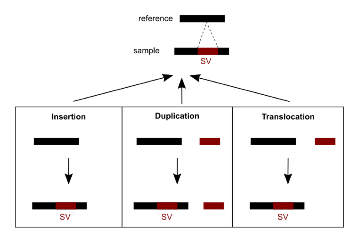
Figure 1: An SV was called for a sequence from a sample differing from the reference sequence. Three possible scenarios of formation could explain the SV observed: an insertion, a duplication or a translocation.
Future of genomic spelling and grammar checkers
Standards and objective benchmarking for SV detection are still missing, so one must be careful with results obtained from current methods. However, SVs are increasingly recognized as being important and technologies to detect them are evolving rapidly. I think their use will become a more common practice in genomic variation studies in a few years, similar to spelling and grammar checkers in text processors. And you, which genome checker will you use?
Reference
Mahmoud M, Gobet N, Cruz-Dávalos DI, Mounier N, Dessimoz C, Sedlazeck FJ. 2019. Structural variant calling: the long and the short of it. Genome Biol 20:246. doi:10.1186/s13059-019-1828-7.
If you want to get involved in improving SV variant detection, consider joining this Hackathon, to be hold remotely Oct. 11-14, 2020.
•
Author: Natasha Glover •
∞
Got newly sequenced genomes with protein annotations? Need to quickly and easily define the homologous relationships between the genes?
OMA Standalone is a software developed by our lab which can be used to infer homologs from whole genomes, including orthologs, paralogs, and Hierarchical Orthologous Groups (Altenhoff et al 2019).
The OMA Standalone algorithm works like this:
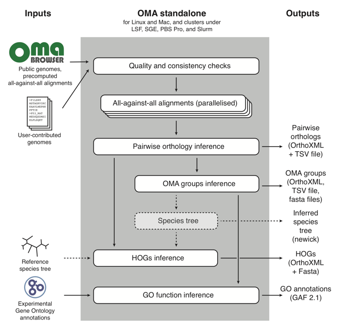
In short, it takes as input user-contributed custom genomes (with the option of combining them with reference genomes already in the OMA database), and proceeds through three main parts:
- Quality and consistency checks of the genomes that will be used to run OMA Standalone;
- All-against-all alignments of every protein sequence to all other protein sequences;
- Orthology inference, in the form of: pairwise orthologs, OMA Groups, and Hierarchical Orthologous Groups (HOGs). For more information on these types of orthologs output by OMA, see OMA: A Primer (Zahn-Zabal et al. 2020).
Although the OMA Standalone is well-documented and straightforward, one of the challenges can be running it on an High Performance Cluster (HPC).
In order to understand the bare necessities needed to run OMA Standalone, we wrote an OMA Standalone Cheat Sheet, which you can download and follow the step-by-step instructions on running the software on an HPC. We use the cluster Wally as an example, as that is one of the HPCs here at the University of Lausanne. Wally uses SLURM as the scheduler for submitting jobs, so all the examples will be shown with that. We plan in the future to provide additional information on running with other schedulers, such as LSF or SGE. In the Cheat Sheet, you will find tips, hints, commands, and example scripts to run OMA Standalone on Wally.
Additionally, we prepared a video which walks the user through the process of running OMA Standalone from start to finish, including:
- Downloading the software
- Preparing your genomes for running
- Editing the necessary parameters file
- Creating the job scripts and
- Submitting your jobs
The video can be found on our lab’s YouTube channel, at OMA standalone: how to efficiently identify orthologs using a cluster, and is also embedded here for your convenience:
We hope these resources can be helpful if you need help getting started running OMA Standalone. But don’t forget, there is also plenty of information that can be found on the OMA Standalone webpage or in the OMA Standalone paper. If all else fails, don’t hesitate to contact us on Biostars.
References
- Altenhoff, A. M. et al. OMA standalone: orthology inference among public and custom genomes and transcriptomes. Genome Res. 29, 1152–1163 (2019).
- Zahn-Zabal, M., Dessimoz, C. & Glover, N. M. Identifying orthologs with OMA: A primer. F1000Res. 9, 27 (2020).
 The Dessimoz Lab
blog is licensed under a Creative
Commons
Attribution 4.0 International License.
The Dessimoz Lab
blog is licensed under a Creative
Commons
Attribution 4.0 International License.